For this watershed, two types of models were created: Model Type B - informed by the statewide big data products; and Model
Type A - that by accurate land surface representation,
but no other big groundwater data. More specifically, while both models
utilize the 10 m DEM, Model Types B apply the spatially-explicit bottom
aquifer elevation, conductivity, and recharge inputs, whereas Model
Types A utilize a single, effective value for conductivity and
recharge for all cells in the model and a constant bottom aquifer
elevation, computed as the minimum DEM elevation minus a user-prescribed
length, Z.
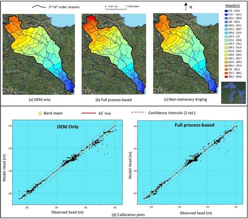
The figure below contains head maps (upper section) generated from (a) Model Type A; (b) Model Type B’ ; and (c) non-stationary kriging (spatial interpolation of data. All head maps share the same color scheme and legend for easy comparisons. Also included are (d) calibration plots (lower section) comparing the results of the Model Types A with SWLs (left-side chart) and similarly for the Model Types B (right-side chart). Confidence intervals of 2 standard deviations and moving window averages (‘band mean’) were computed and added to assist with graphical analysis of the sets of data pairs for each watershed.
Results show that existing data alone enables effective modeling of overall system dynamics. Moreover, of all the existing datasets, those representing topography, lakes, streams and surface seeps are the most important. Digital Elevation Models (DEMs) are especially useful for mapping surface drainage features. In fact, DEM-based treatment of groundwater surface seepage may be the most robust approach for the developing an initial model of a large groundwater system, which can then be used as: 1) a starting point for system-based management; 2) a context to study local perturbations (e.g., geological & stress variability); and 3) a guide for local data collection.