Test Case 1
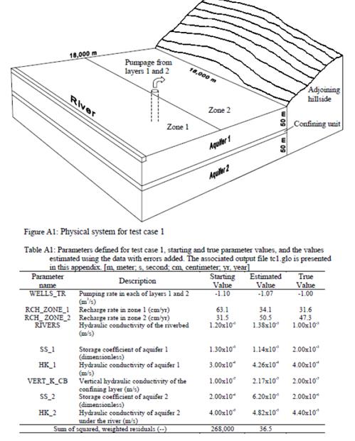
The physical system for test case 1 is shown in figure A1. The system consists of two confined aquifers separated by a confining unit. Each aquifer is 50 m thick, and the confining unit is 10 m thick. The river is treated as a head-dependent boundary that is hydraulically connected to aquifer 1. Recharge from the hillside adjoining the system is treated as a head dependent boundary that is hydraulically connected to aquifers 1 and 2 at the boundary farthest from the river.
Stresses on the system include (1) areal recharge to aquifer 1 in the area near the stream (zone 1) and in the area farther from the stream (zone 2), and (2) pumpage from wells completed in each of the two layers. Pumpage from aquifer 1 is assumed to equal pumpage from aquifer 2. Observations of head and river-flow gain are available for comparison with steady- and transient-state model results. The river is represented using MODFLOW-2000’s River Package.
For the finite-difference method, the system is discretized
into square 1,000-m by 1,000-m cells, so that the grid has
18 rows and 18 columns. Time discretization for the model run is
specified to simulate a period of steady-state conditions
with no pumpage followed by a transient state period with
a constant rate of pumpage. The steady-state period is simulated with
one stress period having one time step. The transient
period is simulated with four stress periods: the first
three are 1, 3, and 6 days long, and each has one time step; the
fourth is 272.8 days long and has 9
time steps, and
each time-step length is 1.2 times the length of the previous time-step
length.
The parameters that define aquifer properties are shown in figure A1 and listed in tables A1 and A2. The hydraulic conductivity of aquifer 2 is known to increase with distance from the river. The variation is simulated using the multiplier-array capability of MODFLOW-2000. In this case, a multiplier array is defined to represent a step function and contains the value 1.0 in columns 1 and 2, 2.0 in columns 3 and 4, and so on to the value 9.0 in columns 17 and 18; this multiplier array is referenced in the definition of parameter HK_2 in the input file for the Layer Property Flow Package. For this test case, parameters SS_1 and SS_2 are defined such that their values are storage coefficients. SS_1 and SS_2 are divided by the aquifer thickness (using a multiplier array defined to be the inverse of the aquifer thickness) to produce the specific-storage values expected by the Layer Property Flow Package.
The river is simulated using the River Package to designate 18 river cells in column 1 of layer 1; the head in the river is 100 m. The conductance of the riverbed for each cell is calculated as ([LRB ´ WRB / bRB] ´ K_RB), where, for each cell, LRB is the length of the river, WRB is the width of the river, and bRB is the thickness of the riverbed. K_RB is a parameter defined to be the hydraulic conductivity of the riverbed material, so that the quantity [LRB ´ WRB / bRB] is listed as Condfact for each cell in the input file for the River Package (Harbaugh and others, 2000). For this system, LRB = 1000 m, WRB = 10 m, and bRB = 10 m at each river cell, so all Condfact values equal 1000 m. Ground-water flow into the system from the adjoining hillside is represented using the General-Head Boundary Package. Thirty-six general-head-boundary cells are specified in column 18 of layers 1 and 2, each having an external head of 350 m and a hydraulic conductance of 1x10⁻⁷ m2/s.
Recharge in zone 1 (RCH_1) applies to cells in columns 1 through 9, recharge in zone 2 (RCH_2) applies to cells in columns 10 through 18. A multiplier array defined as a constant is referenced in the definitions of the recharge parameters to convert the recharge rates from units of cm/yr to m/s.
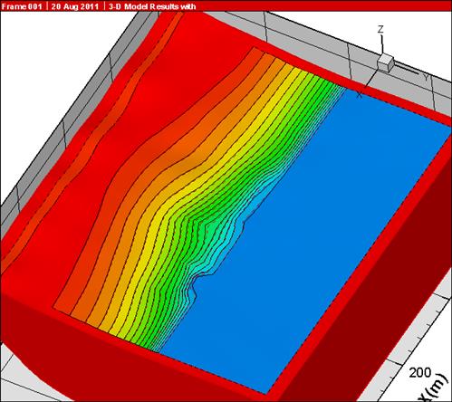
MODFLOW & IGW Comparison
The predicted 3D head distribution by IGW and Modflow matches well.
Legend:
Modflow: Color map and dashed lines
IGW: Black solid lines
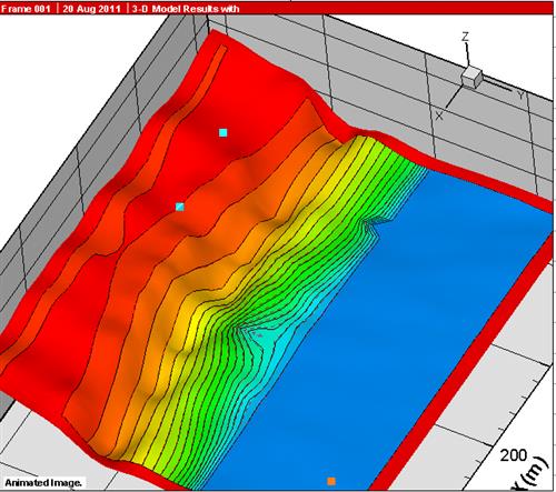
The predicted 3D head distribution by IGW and Modflow matches well.
Legend:
Modflow: Color map and dashed lines
IGW: Black solid lines