Geo-Referenced Pipe Network Model

Login

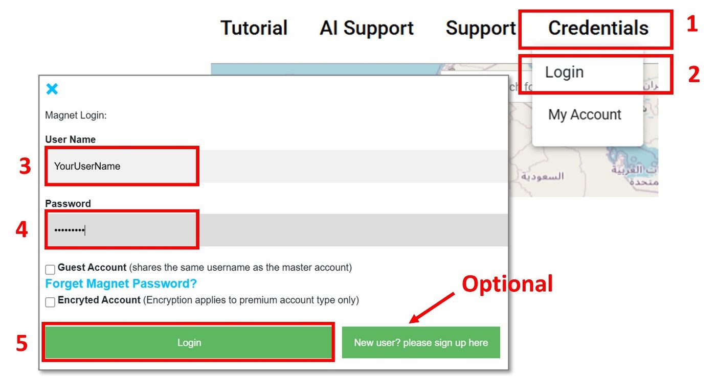
1. Click on ‘Credentials’ on the main toolbar, then click ‘Login’ and enter your Magnet4Water user information

2. If you don’t have a Magnet4Water account, you can click the ‘New user…’ button to sign up.

3. Note: premium users will be asked to verify their accounts to login.

Site Initialization & Conceptual Model

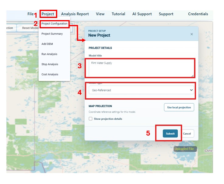
1. Create a new project: File > New Project

   1. Provide a Model Title (e.g. ‘Flint Water Supply’)

   2. Use ‘Geo-referenced’ Model Type

   3. (Optional) Choose to use a local projection by clicking the “Use Local Projection” button.¹

   4. Click ‘Submit’ to save inputs.

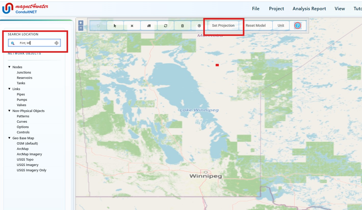
2. Pan and scroll to area of interest in the map display. (Optionally you can use the search bar to search for ‘Flint, MI’) .

3. Develop a Conceptual Model:

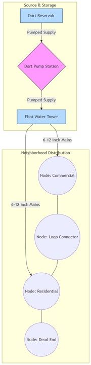
   1. The underground Dort Reservoir, northeast of Flint, stores 20 million gallons of water

   2. Dort Pump Station sends the water from the underground vault to a water tank, and then through the city’s water mains to homes and businesses.

   3. We will use several demand nodes to represent municipal water use.

Add a Reservoir

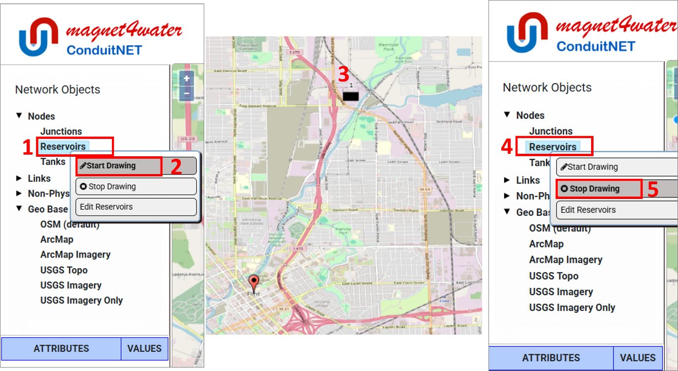
1. Draw the reservoir: Under Network Objects: Nodes > Reservoirs (click, right click) > Start Drawing

   1. Use a single-click to draw the reservoir in the map display.

2. Stop drawing Reservoirs

   1. Nodes > Reservoirs (click, right click) > Stop Drawing, or

   2. Alternatively, “Stop Drawing” for any object can be triggered with the

      

      option on the map toolbar.

3. Edit Reservoir Elevation:

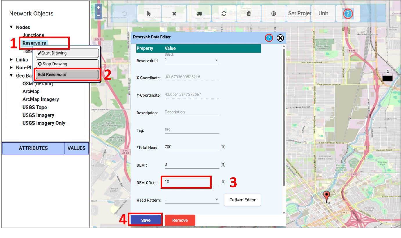
   1. Nodes > Reservoirs (click, right click) > Edit Reservoirs (or just click on the reservoir)

   2. Change the DEM offset to 10ft to indicate reservoir will be below ground, and save. The Total Head will automatically be changed when DEM values are added later.

Add a Tank

1. Zoom in to the area where you placed the reservoir

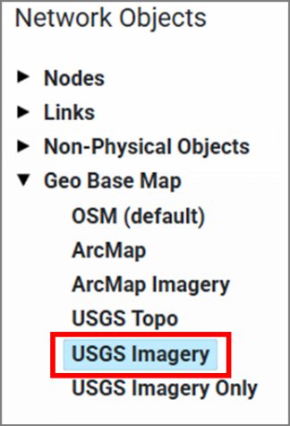
2. Change the basemap display to an aerial imagery view: Under Network Objects > Geo Base Map > USGS Imagery (or ArcMap Imagery)

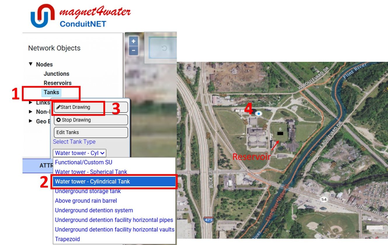
3. Draw the tank coinciding with its location on the map.²

1. Under Network Objects: Nodes > Tanks (click, right click)

   1. Select Tank Type as ‘Water Tower - Cylindrical Tank’

   2. Click ‘Start Drawing’

2. Use a single-click to add the tank over the white oval on the map

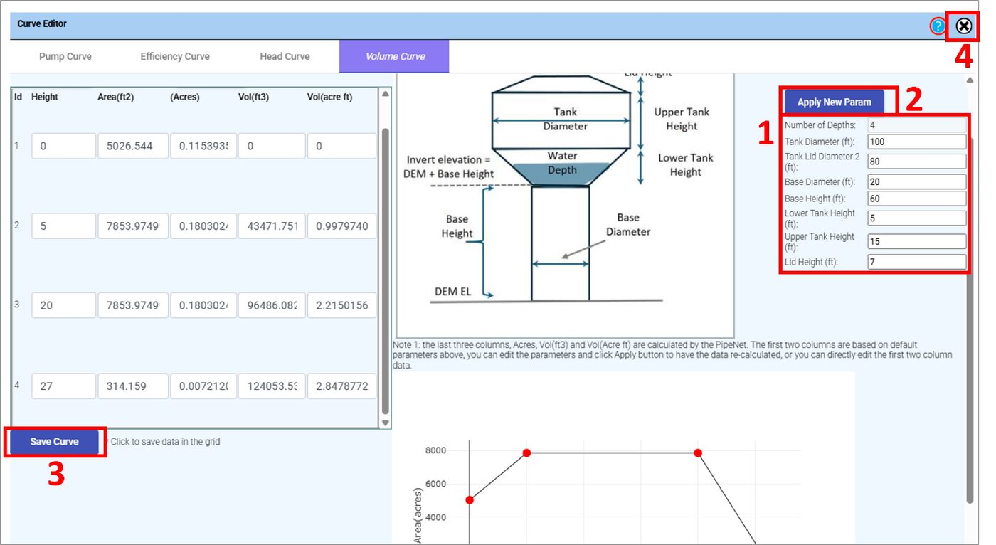
4. Drawing a predefined tank type will automatically display the curve editor³. Edit the parameters here

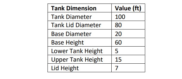
1. Set the tank diameters and heights.

2. Click ‘Apply New Param’ to update the depth volume curve

3. Click ‘Save Curve’

4. Close the Curve Editor

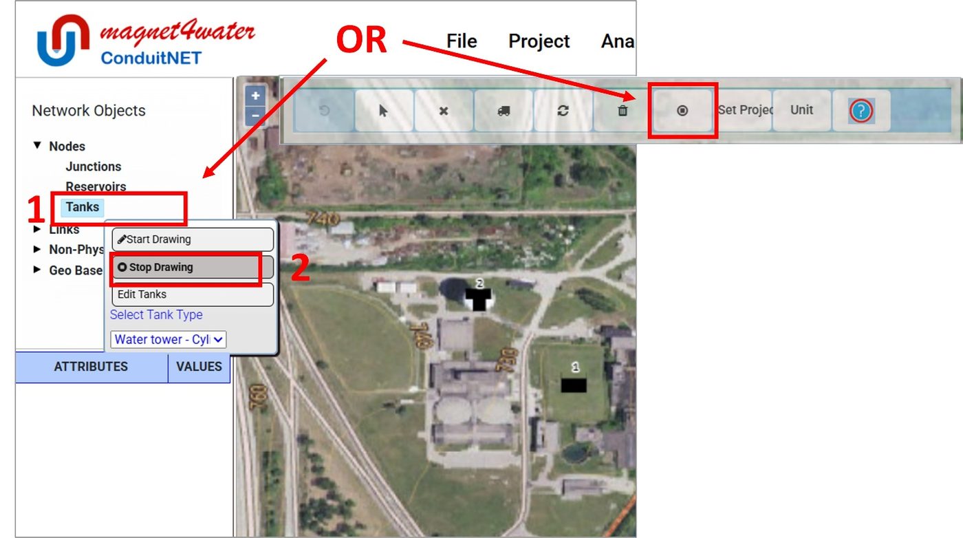
5. Stop drawing Tanks: Nodes > Tanks (click, right click) > Stop Drawing (or click ‘Stop Drawing’ on the map toolbar).

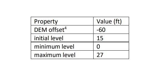
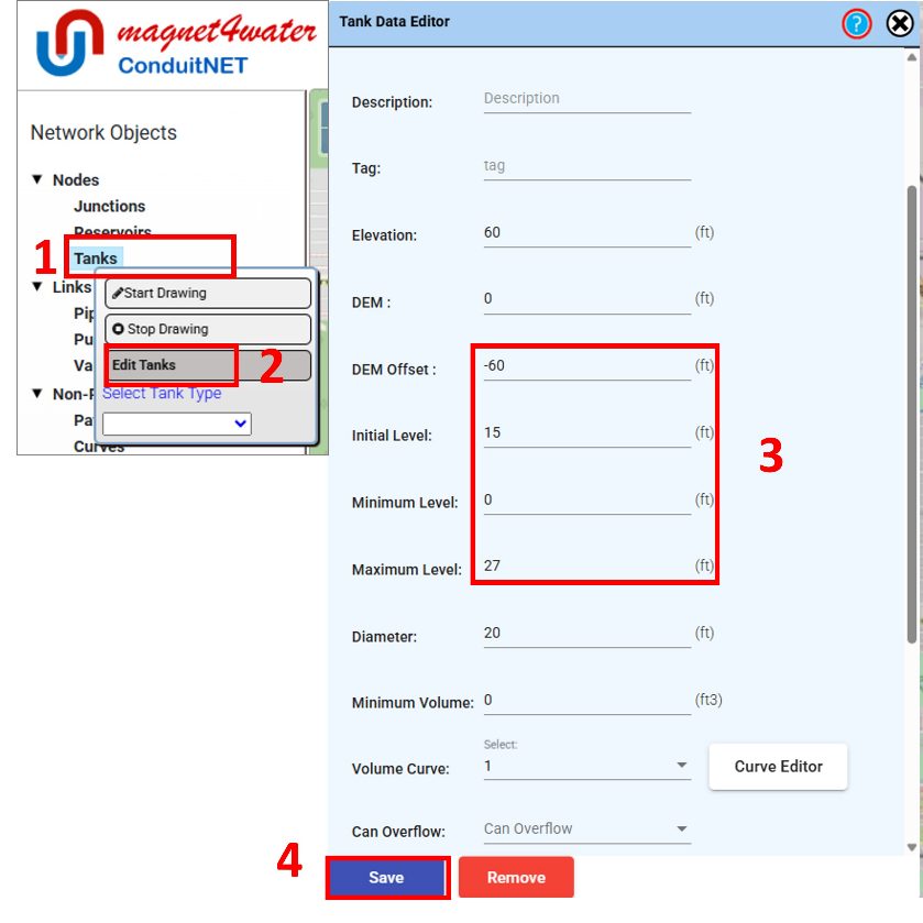
6. Edit tank heights and elevations

1. Nodes > Tanks (click, right click) > Edit Tanks (or just click on the tank)

2. Ensure tank properties are consistent with those used in the Curve editor.

3. Save and close Tank Data Editor.

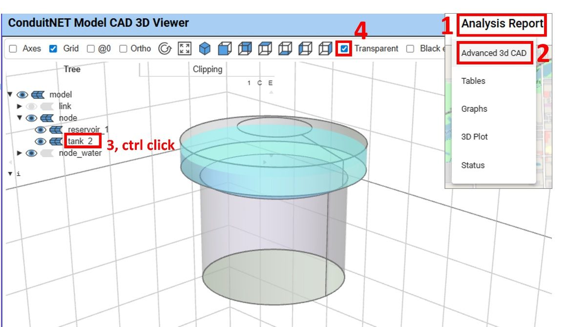
4. (Optional) View a representation of the tank in 3D CAD view

   • Generate a CAD rendering: Analysis Report > Advanced 3D CAD

   • Zoom to the tank: Expand the “model” > “node” tree view on the left, then hold “ctrl” and click on “tank_2”

   • Explore the tank geometry, note the “Transparent” toggle allows visualizing the initial water level inside the tank.

   • The 3D CAD view can be used at any time for a digital twin representation of the pipe network created in ConduitNET.

Add Junction(s)

1. Change base map back to default: Under Network Objects > Geo Base Map > OSM (default)

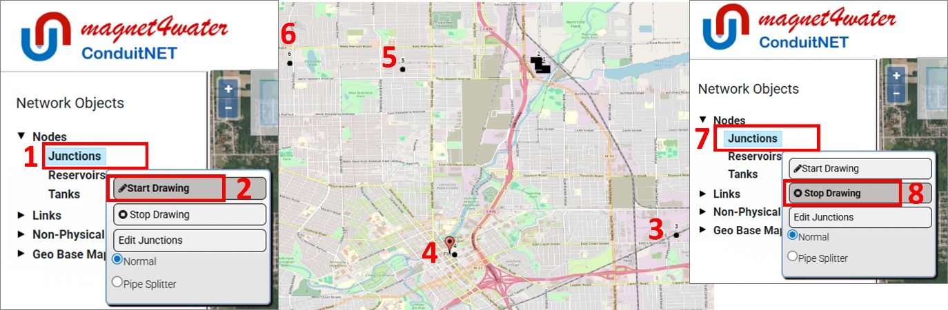
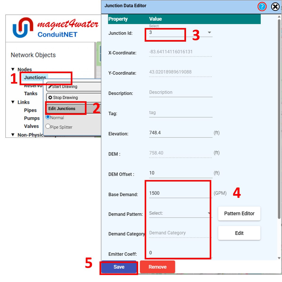
2. Under Network Objects: Nodes > Junctions (click, right click) > Start Drawing

1. Use a single-click to add the 4 junctions to the map (see below).

2. Commercial, commercial/residential, residential, residential dead end

3. Stop drawing junctions: Nodes > Junctions (click, right click) > Stop Drawing

Link the Reservoir and the Tank with a Pump

1. Zoom in to the location with the reservoir and tank

2. Under Network Objects: Links > Pumps (click, right click) > Start Drawing

   1. Click once on the Reservoir to snap the pump’s starting position to it. A blue line will extend from the node as you move the cursor.

   2. Double click on the tank to snap the pump’s ending position to it.⁵

3. Stop drawing pumps: Links > Pumps (click, right click) > Stop Drawing

Link the Tank and Junctions together with Pipes

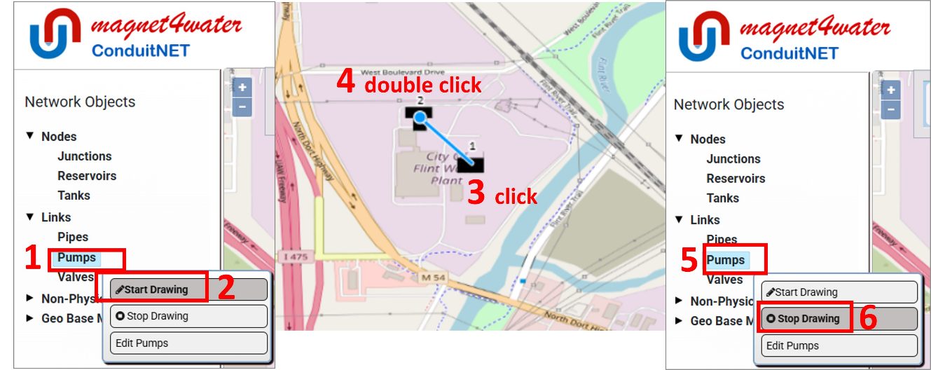
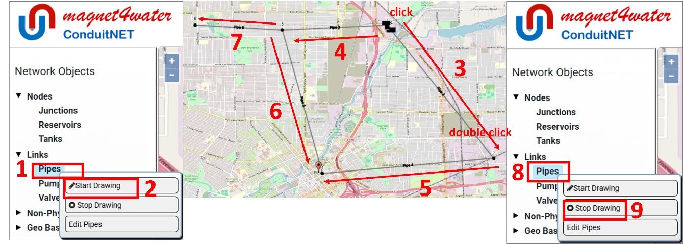
1. Under Network Objects: Links > Pipes (click, right click) > Start Drawing

   1. Click once on the tank to snap the pipe’s starting position to it. A blue line will extend from the node as you move the cursor.

   2. Double click on the southeast junction to snap the pipe’s ending position to it.

   3. Repeat (i) and (ii) four more times to link all the nodes following the diagram below. Remember to start each pipe at the tail end of the arrow and finish at the head. When completed you should have links ‘Pipe 2’ to ‘Pipe 6’

2. Stop drawing Pipes: Links > Pipes (click, right click) > Stop Drawing

Get Object Elevations from DEM

1. Project > Add DEM

2. After a short while, the Elevations for all Node objects (the reservoir, tank, and junctions) will be automatically updated based on DEM.⁶

3. (Optional) Click on a node object (e.g., tank) to see updated ‘Elevation’.

Update Junction Properties

1. Under Network Objects: Nodes > Junctions (click, right click) > Edit Junctions (or just click on any junction)

2. Update the Base Demand and Emitter Coefficient⁷.

   1. ‘Save’ the junction properties

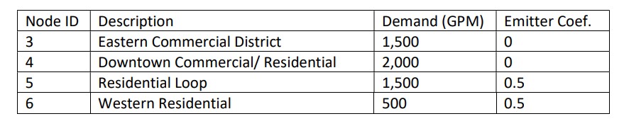
   2. Repeat for each junction to match the table below.

3. You can toggle between different junctions by using either the Junction Id dropdown in the Junction Data Editor or by closing the Editor and clicking on a different junction.

Update Pipe Properties

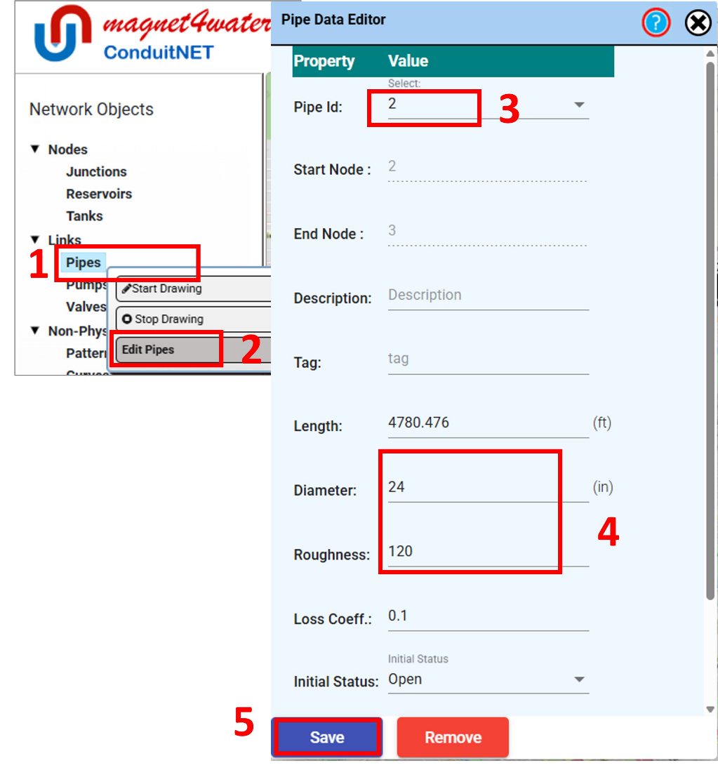
1. Open the Pipe Editor, under Network Objects: Links > Pipes (click, right click) > Edit Pipes (or just click on any pipe)

2. Set the diameter for all pipes to 24 inches, and the roughness to 120.

3. Save parameters for each pipe before changing to the next. You can toggle between different pipes by using either the Pipe Id dropdown in the Pipe Data Editor or by closing the Editor and clicking on a different pipe.

Update Pump Properties

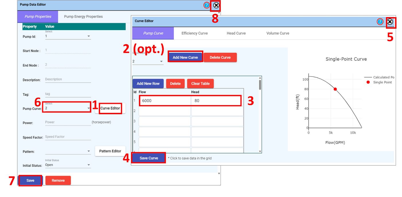
1. Open the Pump Data Editor, under Network Objects: Links > Pumps (click, right click) > Edit Pumps (or just zoom in and click on the pump between the reservoir and the tank)

2. Click on ‘Curve Editor’ to open the Curve Editor. Make sure the ‘Pump Curve’ tab is selected.

3. (If no pump curve exists) Click ‘Add New Curve’ to generate a new pump curve.

4. Enter a flow rate of ‘6000’ GPM, and a head of ’80’ feet then click ‘Save Curve’, and close the Curve Editor.

5. Back on the Pump Data Editor, ensure that the curve you just modified/created is selected from the ‘Pump Curve’ dropdown, click ‘Save’, and close the Pump Data Editor.

Check Analysis Settings

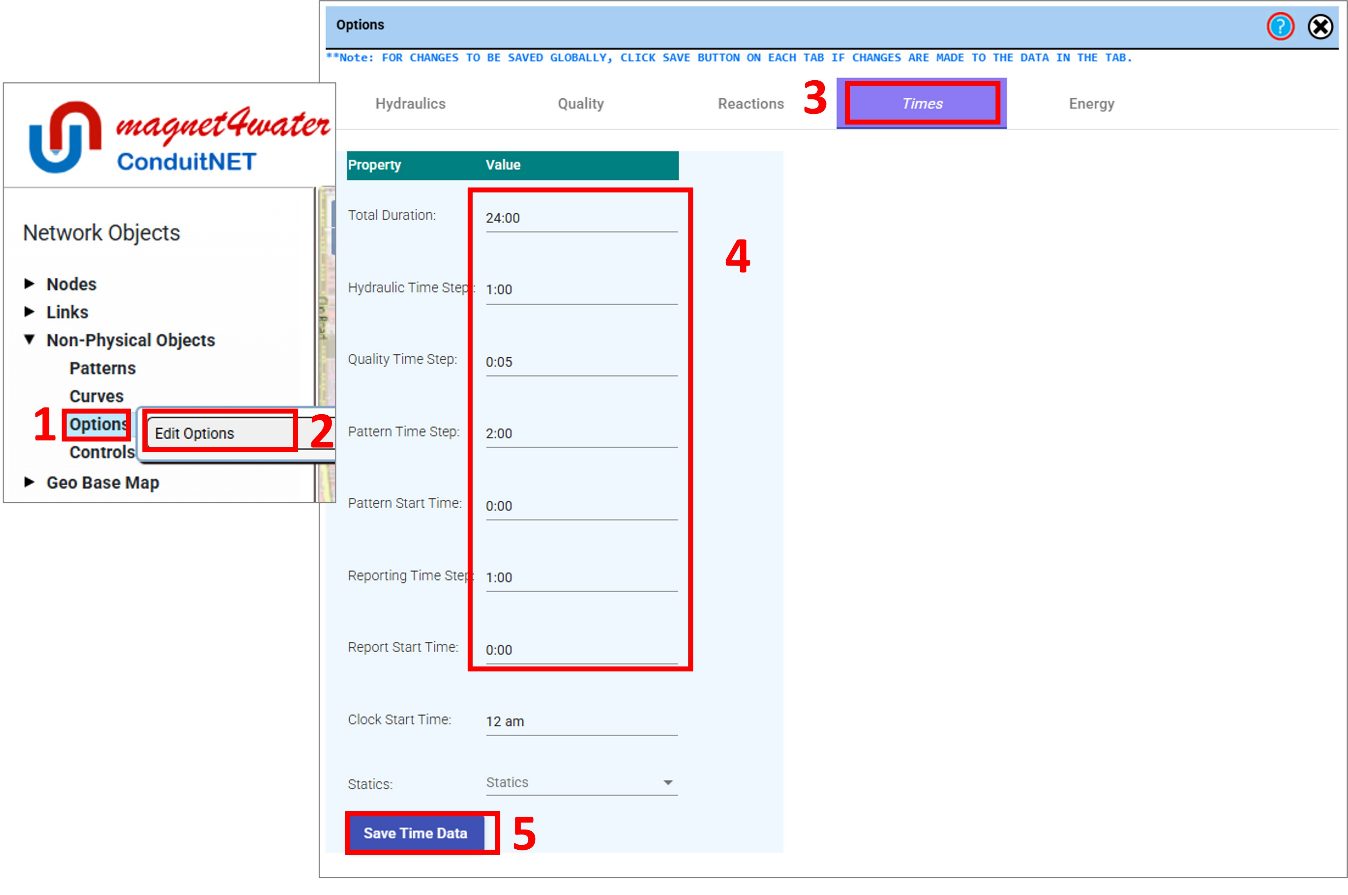
1. Under Network Objects: Non-Physical Objects> Options (click, right click) > Edit Options

2. Default may be used.

3. Confirm values on the Times tab

   1. Ensure duration is 24:00

   2. If any changes are made ‘Save Time Data’ and then close the Options dialog.

Save Model and Run Analysis

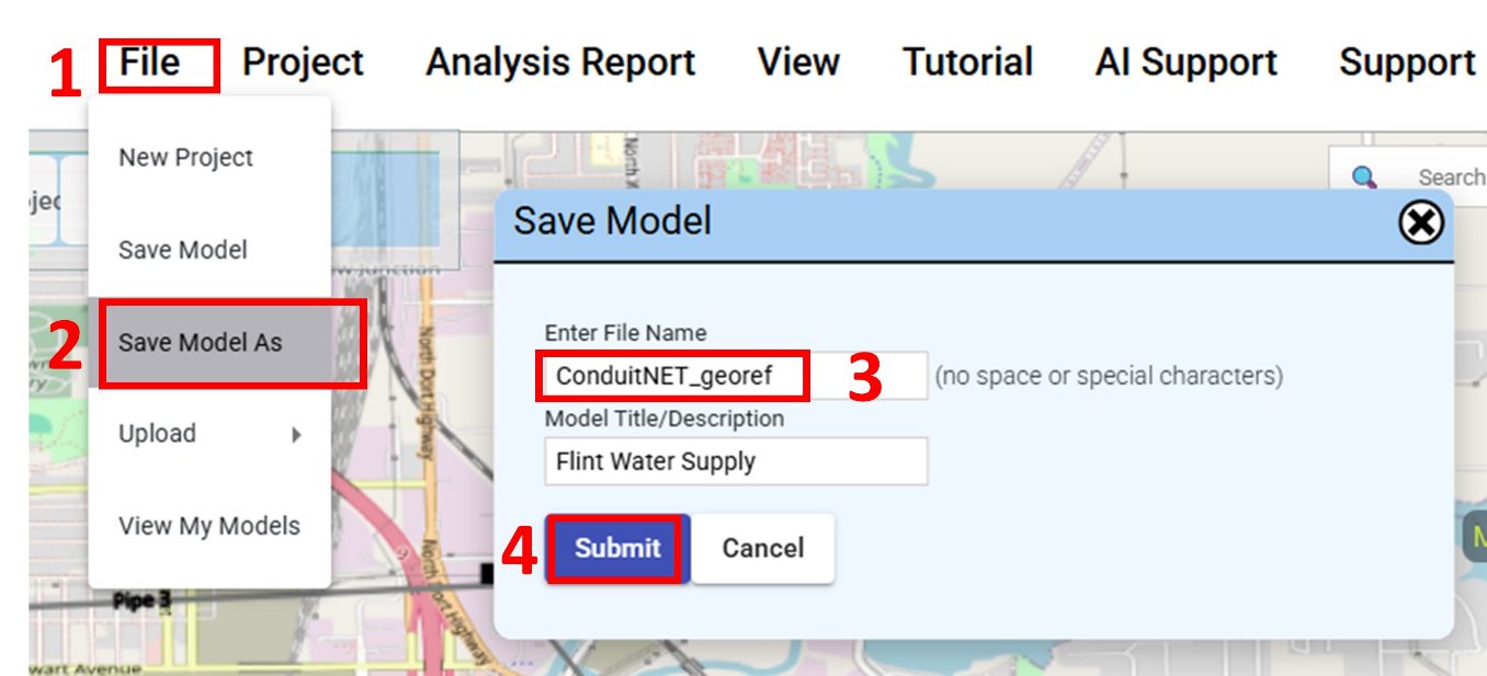
1. Save the changes to the model: File > Save Model As⁸

   1. Enter file name and `Submit`

   2. If the number of models saved exceeds your user limit, you can upgrade, or delete unused model files.

2. Submit the model for simulation:

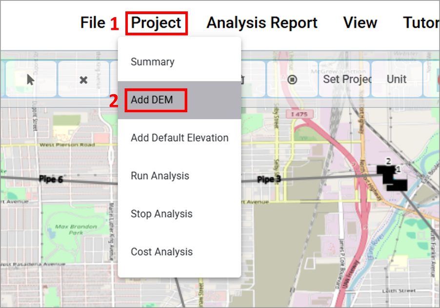
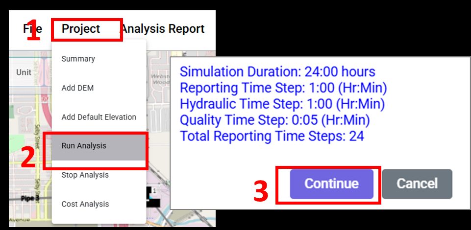
   1. Project > Run Analysis

   2. After a moment a dialog should pop up giving the analysis duration as 24 hours with 24 reporting time steps. Click ‘Continue’

3. After the model is executed, the Status Window⁹ will appear.

   1. If you close the Status Window and want to view again: Analysis Report > Status

View Plan View Results

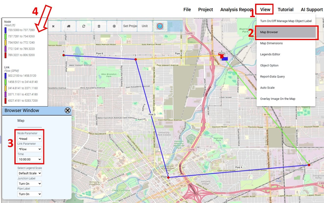
1. By default, plan-view results will presented as color-coded reservoirs, tanks, junctions, and pipes, with legends to indicate the range of values corresponding to each color¹⁰.

2. Use the Browser Window to explore results for different node and link parameters at different times.

   1. If you close the Browser Window and want to use it again: View > Map Browser.

3. Inspect the legend and map to see model output values.

View Time-series Results

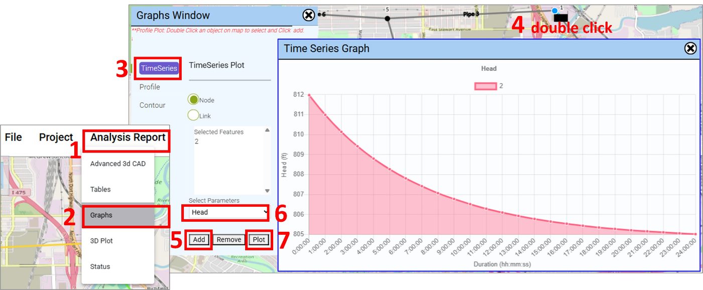
1. Analysis Report > Graphs

2. In the Graphs Window, click ‘TimeSeries’:

   1. Select ‘Node’ as the Object Type

   2. Double-click on the tank in the map display

   3. Click the `Add` button to add the tank ID to the Selected Features ID List¹¹

   4. Select ‘Head’ as the Parameter

   5. Click ‘Plot’

3. A Plot will automatically appear showing the head results in the tank (and any other selected nodes) over the entire analysis duration.

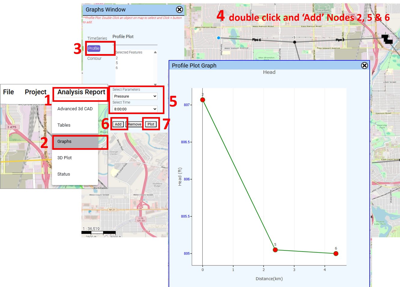
View Results along a Profile

1. Open the Graphs Window (see above, Analysis Report > Graphs)

2. In the Graphs Window, click ‘Profile’:

   1. Double-click on the tank in the map display

   2. Click the `Add` button to add the tank ID to the Selected Features ID List

   3. Repeat step ii and iii to click on adjacent nodes in order (junctions 5 and 6)

   4. Select ‘Head’ or another Parameter

   5. Select a given Time from the dropdown

   6. Click ‘Plot’

3. A Plot will automatically appear showing the head (or other parameter) results along the selected nodes at the selected time. Note how head and pressure change along the profile.

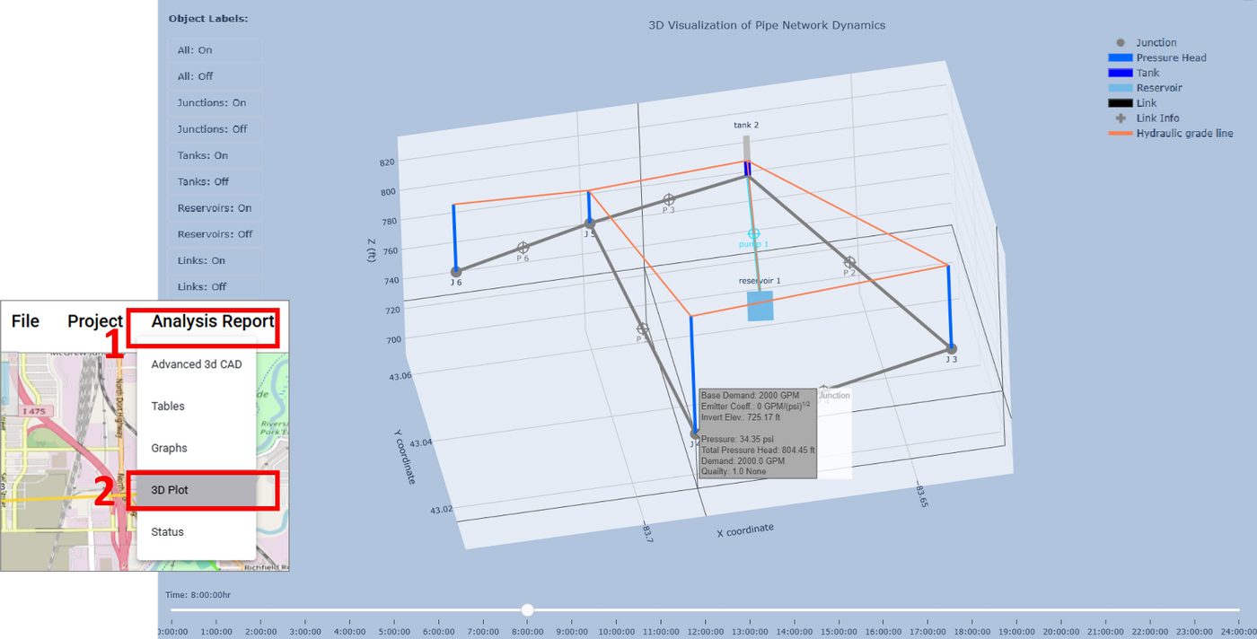
View 3D results

1. To display the model results in 3D:

   1. Analysis Report > 3D Plot: this will open a new window with the 3D plot.

   2. The mouse may be used to rotate/zoom the plot, and the left panel controls to toggle feature labels on and off.

   3. Use the time slider on the bottom to see analysis results over time.

   4. Hover over any link or node object to view object properties, and calculated values at the current slider time.

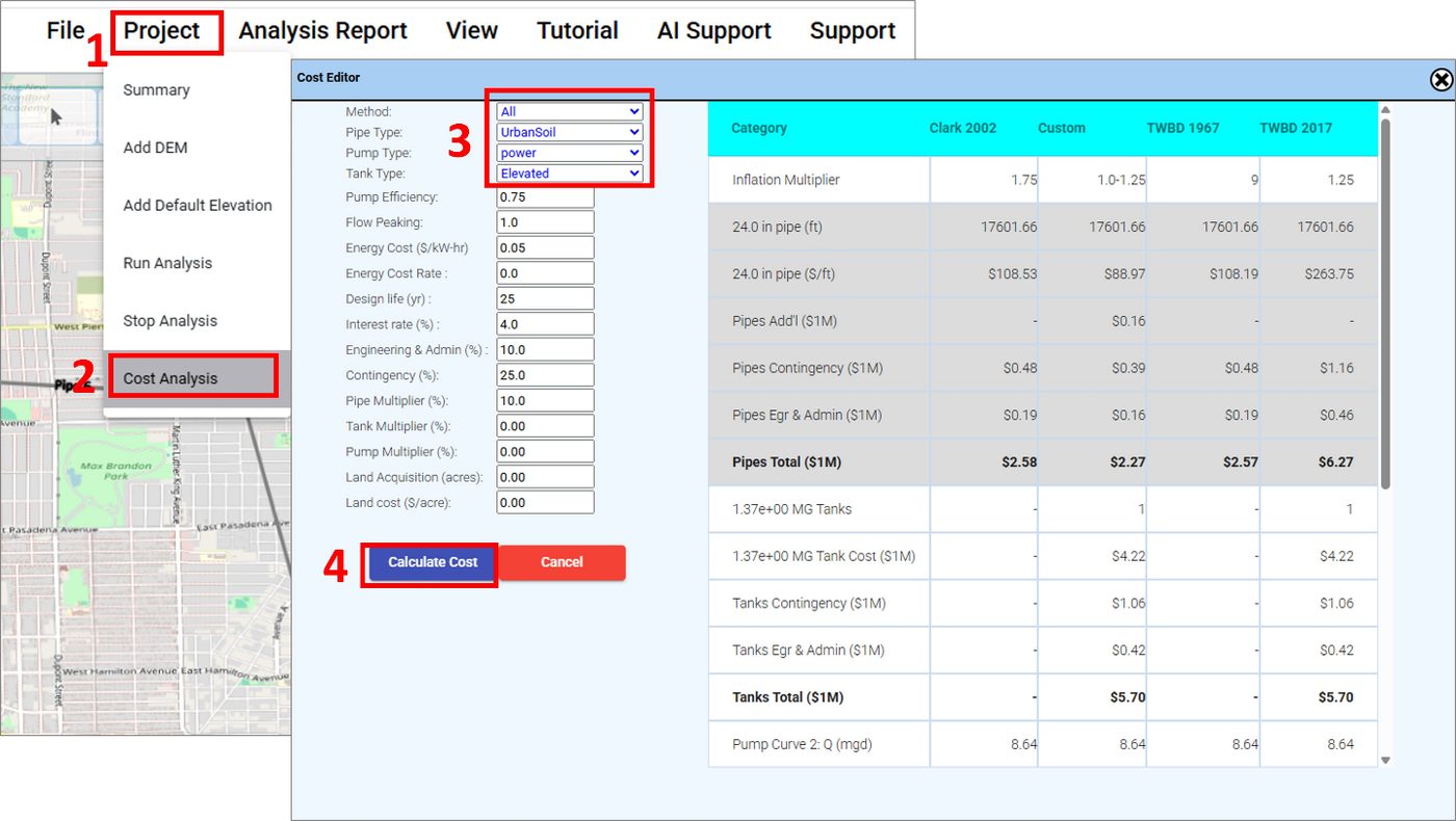
Calculate Network Cost Estimates

1. To estimate pipe network costs:

   1. Project > Cost Analysis

   2. Change pipe type to ‘urban soil’

   3. Click ‘Calculate Cost’

REFINING THE MODEL

Change the demand pattern

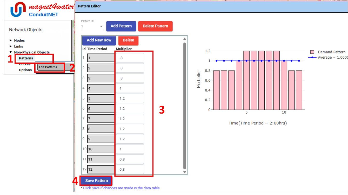
Water usage is higher during the day and lower at night. Update the demand pattern to reflect this.

1. Under Network Objects: Non-Physical Objects> Patterns (click, right click) > Edit Patterns

2. The pattern starts at 12am and runs for 24hr (see Times Options in section 12 above).

3. Decrease demand multiplier to 0.8 from 1 – 3 (12am to 6 am), and 11 – 12 (8pm to 12am)

4. Increase demand multiplier to 1.2 from 5 – 9 (6am to 8pm)

5. Click ‘Save Pattern’ and close the Pattern Editor

Optional Refinements

1. Add additional junctions and links to make a more complex and representative network.

2. Change pipe sizing and see the impact on head, pressure, and cost.

3. Model contaminant flow through the system.

4. Experiment with control rules to tun on/off pumps and/or open/close links based on parameters.

Save Model, Re-Run Simulation, and View Results

1. Save and run the refined model (See Section 13)

2. Confirm that the analysis includes the model demand refinements:

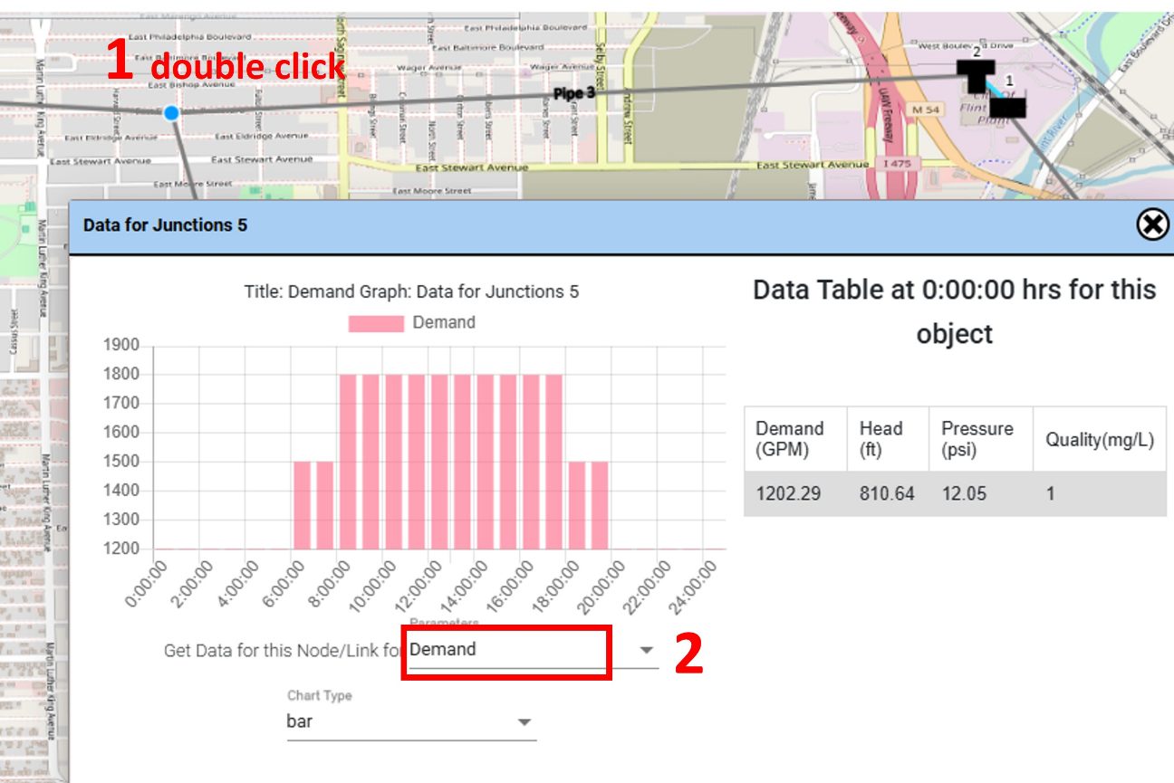
   1. Double click on one of the junctions to open the object data viewer.

   2. Select ‘Demand’ from the ‘Get data for this Node/Link for’ dropdown.

   3. Confirm that demand varies from 0.8 to 1.2 time the demand listed in table in Section 9 (e.g., for junction 5, original demand was 1500 GPM, new demand varies from 1200 to 1800 GPM).

Solving and Reporting Issues

1. In addition to this tutorial, if the user runs into challenges, ConduitNET has a built in AI Support feature. After clicking AI Support, the user can type questions like “How to write a control rule in ConduitNET”

2. If issues are encountered within ConduitNET, or the user has special requirements, please contact us. Support > Contact Us.