Real World Heterogeneity | MAGNET4WATER Curriculum

01 Salt River Bed, Arizona - 1

What does an aquifer actually look like — if you could see underground?

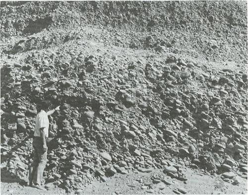
What you’re watching A photograph of a real outcrop in the Salt River bed, Arizona, exposing the sand and gravel of an aquifer formation; people in the frame give a sense of scale, and fine-textured lenses are visible within the coarser sediment.

The mechanism Outcrops let us see directly what is normally hidden. This one shows an aquifer is not a uniform block but a fabric of sands and gravels with embedded finer lenses — the heterogeneity that controls flow and transport, exposed to the eye.

Key relationshipReal aquifers are visibly heterogeneous — layered sands and gravels with finer lenses, not uniform material.

Why it matters Seeing the real thing grounds every model: the heterogeneity drawn in a simulation is a stand-in for textures like these, which a borehole only samples at points.

IGW-NET This is the real heterogeneity the random-field tools represent — the photograph is the ground truth behind the generated conductivity fields.

02 Salt River Bed, Arizona - 2

How fine can the layering get?

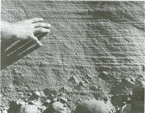
What you’re watching A closer view of the Salt River sediments showing microstratification — many thin laminae of contrasting grain size stacked on top of one another.

The mechanism Sediments are deposited in layers, so heterogeneity is often strongly layered in the vertical direction — down to millimeter- and centimeter-scale laminae. This fine vertical structure is the rule in water-laid deposits.

Key relationshipVertical heterogeneity is often finely layered — microstratification at the centimeter scale and below.

Why it matters These thin layers are far too fine to map individually, yet, as the next panel shows, their cumulative effect on flow is large.

IGW-NET Such fine layering is exactly what an effective vertical conductivity must summarize — the bridge from visible laminae to a usable model parameter.

03 Salt River Bed, Arizona - 3

How does fine layering you can barely see create large-scale anisotropy?

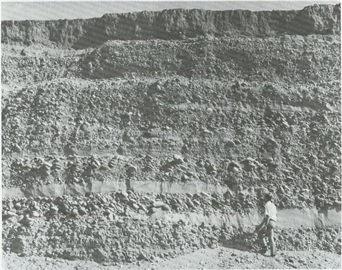
What you’re watching The layered Salt River sediments again — alternating coarser and finer beds — the structure that turns small-scale layering into directional behavior at the aquifer scale.

The mechanism Even if each thin layer is itself isotropic, stacking layers of contrasting conductivity makes the bulk aquifer anisotropic. Horizontal flow runs along the layers, so the effective horizontal conductivity is close to the arithmetic average — dominated by the most permeable beds. Vertical flow must cross every layer in series, so the effective vertical conductivity is close to the harmonic average — dominated by the least permeable bed. The arithmetic average is always greater than the harmonic, so horizontal K ends up much larger than vertical K.

Key relationshipLayered heterogeneity creates anisotropy: horizontal K ≈ arithmetic average (set by the most permeable layers), vertical K ≈ harmonic average (set by the least permeable) — and arithmetic always exceeds harmonic.

Why it matters A single near-impervious layer can throttle all vertical flow while barely affecting horizontal flow — which is why layered aquifers are so strongly anisotropic, and why small-scale heterogeneity must be understood, not ignored.

IGW-NET It reframes anisotropy as a consequence of heterogeneity, not a separate property — the smaller-scale layering you see here is what large-scale anisotropy is made of.

04 Sand & Gravel Aquifer, Swizerland

Does layering only happen at fine scales?

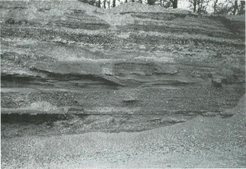
What you’re watching A photograph of a sand-and-gravel aquifer outcrop in Switzerland, showing thicker, distinct beds of differing texture as well as finer internal structure.

The mechanism Heterogeneity exists at many scales at once: here, thicker depositional units each contain their own finer layering. The same arithmetic/harmonic logic applies at every scale, compounding the anisotropy.

Key relationshipLayering occurs across scales — thick beds containing fine laminae — each scale adding to the bulk anisotropy.

Why it matters Real characterization must decide which scales to resolve; the unresolved finer layering still shapes the effective properties.

IGW-NET Seeing nested bed structure in a real outcrop motivates the multiscale heterogeneity the simulations explore.

05 Roswell Basin, New Mexico

Do real aquifer water levels hold steady — or track the wetness of each year?

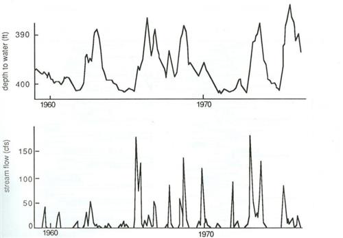
What you’re watching Time-series data from the Roswell Basin, New Mexico: the depth to water (top) rises and falls in step with the stream flow (bottom) over two decades — water levels closely tracking recharge.

The mechanism Real aquifers vary in time as well as space. Years of high stream flow recharge the aquifer and the water table rises (depth to water shrinks); dry years let it fall. The water level becomes a running record of recharge.

Key relationshipAquifer water levels track recharge over time — rising in wet years, falling in dry ones.

Why it matters A reminder that heterogeneity is not only spatial: real systems are forced by time-varying recharge, and water-supply planning must account for these swings.

IGW-NET Time series like this are the real temporal forcing behind the transient and seasonal-variability simulations.

06 Mt. Simon Aquifer, Illinois

If an aquifer is called ‘relatively homogeneous,’ is its conductivity actually uniform?

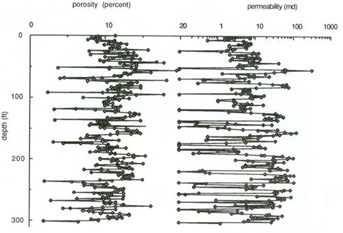
What you’re watching Data from the Mt. Simon aquifer, Illinois — a sandstone considered relatively homogeneous — showing that, measured in detail, its hydraulic conductivity still varies by orders of magnitude.

The mechanism Detailed sampling reveals what ‘homogeneous’ hides: even a clean, uniform-looking aquifer has K spanning orders of magnitude when you have enough data to resolve it. Porosity varies too, though over a much narrower range than K.

Key relationshipEven a ‘relatively homogeneous’ aquifer has K varying by orders of magnitude — porosity varies too, but far less.

Why it matters It is the empirical proof that heterogeneity is the rule: the label ‘homogeneous’ means ‘we haven’t sampled finely enough to see the variation,’ not that none exists.

IGW-NET Real K data like this is what justifies treating conductivity as a random field even for ‘clean’ aquifers.

07 Borden Aquifer -1, Canadan

How variable is the most intensively studied ‘uniform’ aquifer of all?

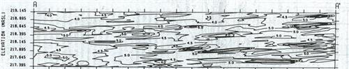
What you’re watching Data from the Borden aquifer, Canada — one of the most densely sampled aquifers in the world — mapping its conductivity in fine detail.

The mechanism Borden is the research benchmark for a near-uniform sand. Even so, its ln K varies measurably from point to point — famously an ln K variance of only about 0.3, which made it the standard against which heterogeneity theory was tested.

Key relationshipBorden is about as uniform as nature gets — ln K variance only ~0.3 — yet it is still measurably variable.

Why it matters If the cleanest aquifer on record is this variable, every practical site is more so — the honest baseline for modeling.

IGW-NET Borden’s measured field is the real data behind the random-field and macrodispersion demonstrations.

08 Borden Aquifer -2, Canadan

What does the structure of that variability look like?

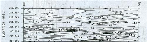
What you’re watching A second Borden view emphasizing the spatial structure — how nearby measurements resemble each other, defining a correlation scale.

The mechanism Beyond the variance, the data reveal spatial correlation: conductivity varies, but smoothly over a characteristic distance. This is exactly the statistical structure — variance plus correlation — that a random-field model needs.

Key relationshipReal data show both a variance and a correlation scale — the two statistics that define a random field.

Why it matters It connects field reality to the modeling tools: outcrops and datasets supply the variance and correlation that simulations then use.

IGW-NET Measured structure like this is what the random-field generators are calibrated to reproduce.