MAGNET Storm Water Network Analysis
TUTORIAL – Georeferenced Model
This is a “generic” tutorial demonstrating how to zoom into any location and create a georeferenced stormwater/urban catchment model. The process is illustrated for a simple network containing the following elements: one subcatchment, one junction, one link, one storage unit, one weir and one outfall. The model results are analyzed for a 24-hour, 100-year Type II SCS storm event. Then the model is refined by modifying the infiltration method, evaporation, groundwater seepage, and water quality (one land use and one pollutant), and adding a second subcatchment with a Low Impact Development (LID) Control.
This tutorial provides graphics for a hypothetical site in Haslett, Michigan, United States, but can be applied at any location.
Steps covered in this Tutorial:
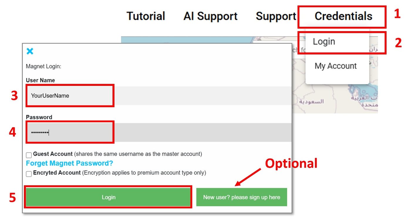
Login
Click on ‘Credentials’ on the main toolbar, then click ‘Login’ and enter your Magnet4Water user information
If you don’t have a Magnet4Water account, you can click the ‘New user…’ button to sign up.
Note: premium users will be asked to verify their accounts to login.
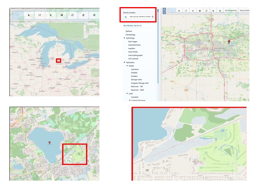
Site Initialization & View Map Layers
Pan and scroll to area of interest in the map display. (Optionally you can use the search bar to search for ‘Lake Lansing, MI’) .
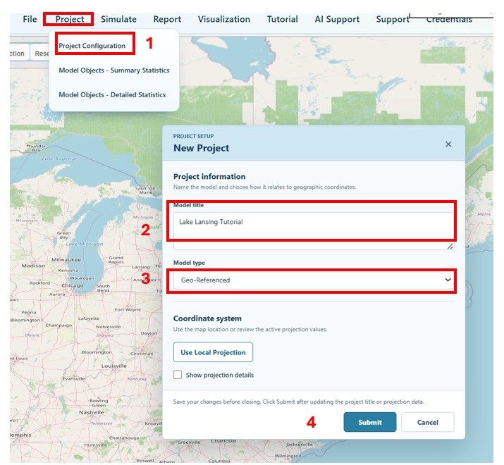
Create a new project: Project > Project Configuration
Provide a Model Title
Use ‘Geo-referenced’ Model Type
(Optional) Choose to use a local projection by clicking the “Use Local Projection” button.1
Click ‘Submit’ to save inputs.
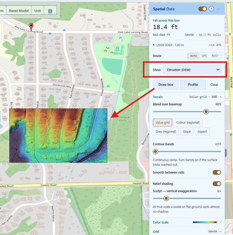
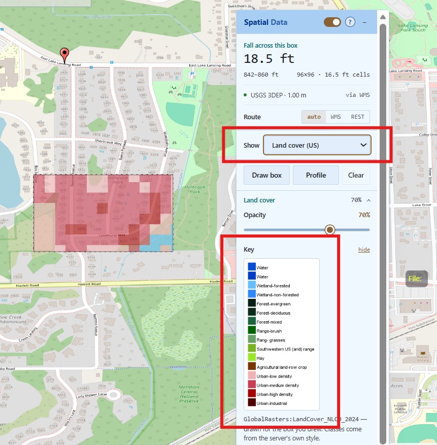
Define a model area and view data layers: after loggin in, you will see the Spatial Data panel on the right side of the map.
Utilize the Spatial Data Panel:
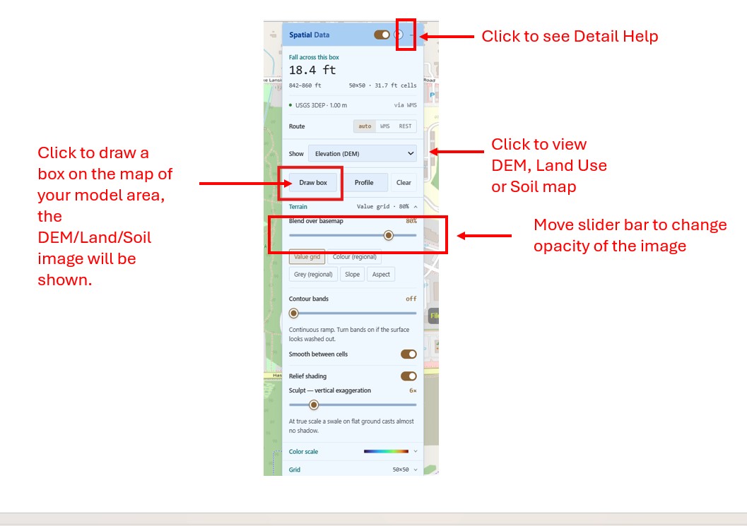
Draw a rectangular box to define the data extraction area.
Click ‘Draw Box’
A single click (e.g. lower left) starts the box, a second click (e.g. upper right) “submits” it
After a short while, the data layers will appear in the map display3
Add a Subcatchment
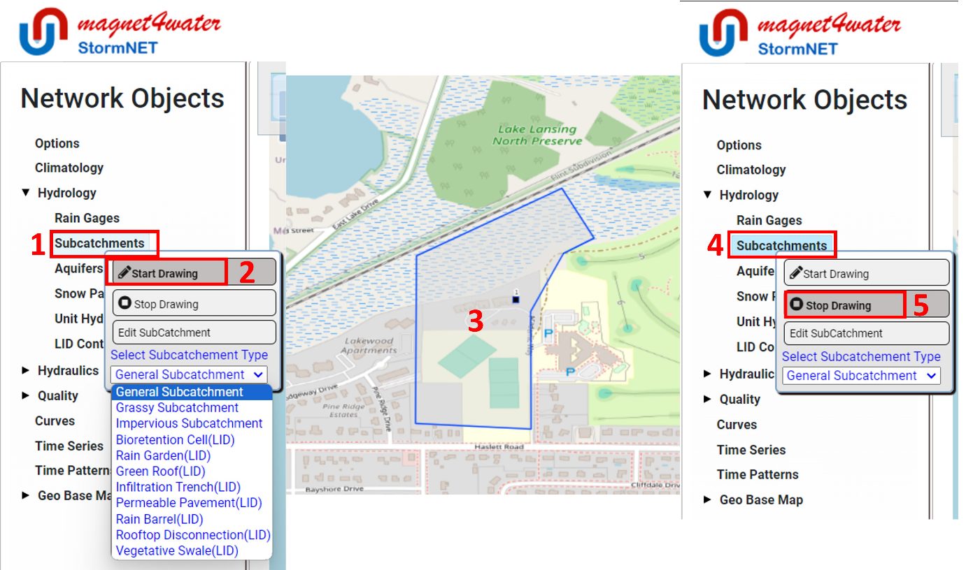
Draw the subcatchment: Under Network Objects: Hydrology > Subcatchments (click, right click) > Start Drawing
(optional) Change the ‘Subcatchment Type’ and click ‘Start Drawing’ again to set visualization and/or low impact development (LID) defaults for subsequently draw subcatchment(s).
Use single-clicks to draw a subcatchment in the map display.
Use a single-click on the previously placed ‘first vertex’ to ‘end’ the drawing and finalize the polygon5
Stop drawing subcatchments
Hydrology > Subcatchments (click, right click) > Stop Drawing, or
Alternatively, “Stop Drawing” can be triggered for any object with the map toolbar.
Add a Junction
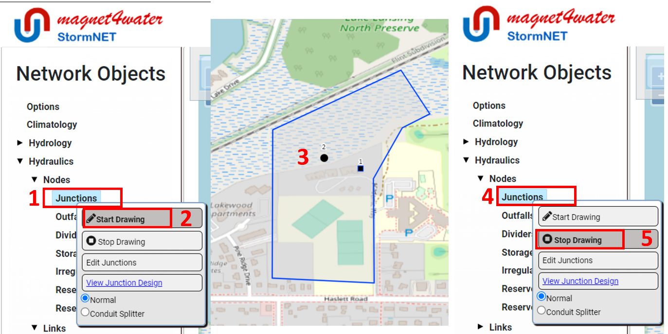
Under Network Objects: Hydraulics > Nodes > Junctions (click, right click) > Start Drawing
Use a single-click to add the junction to a place on the map
Stop drawing junctions: Hydraulics > Nodes > Junctions (click, right click) > Stop Drawing
Connect a Subcatchment to a Junction
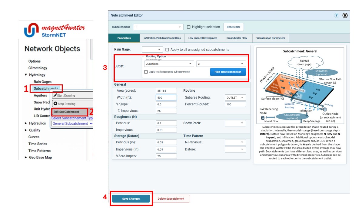
Open the Subcatchment Editor:
single-click on the subcatchment polygon, OR
Hydrology > Subcatchments (click, right click) > Edit SubCatchment
Confirm Subcatchment ‘1’ is selected in Subcat. Id/Name
Select ‘Junctions’ and ‘2’ options next to Outlet
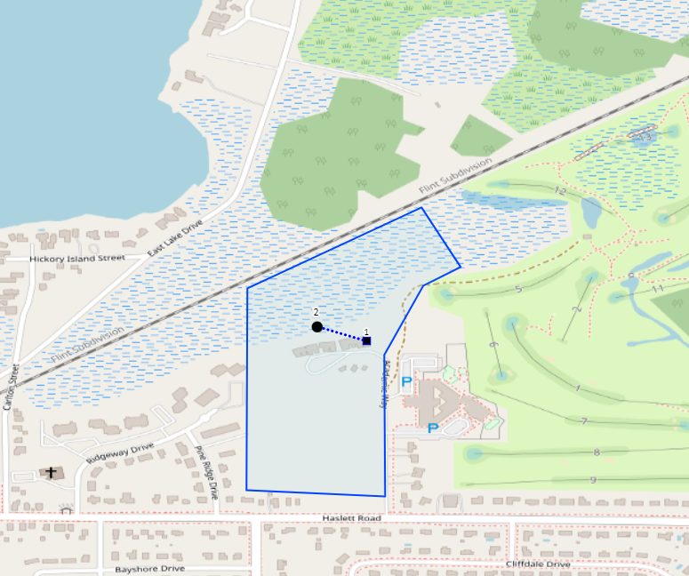
Click ‘Save Subcatchment Data’ and exit the Subcatchment Editor (there should now be a dashed line connecting the subcatchment centroid and the selected junction)
Add a Storage Unit (SU)
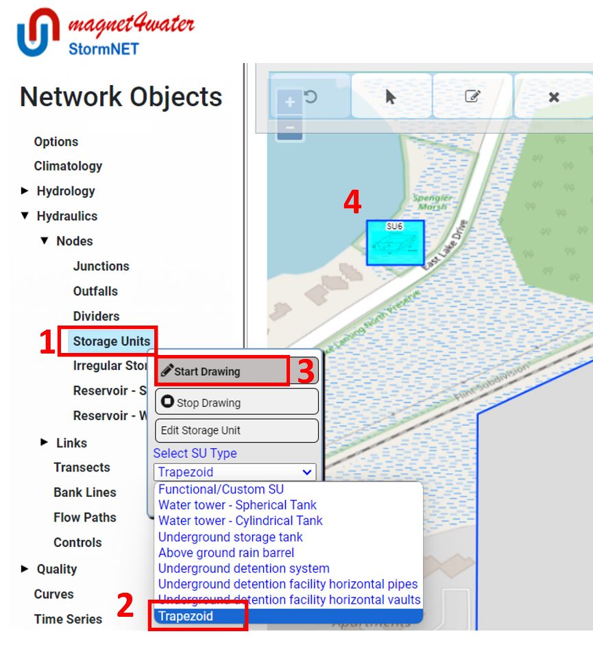
Under Network Objects: Hydraulics > Nodes > Storage Unit (click, right click)
Select SU Type as “Trapezoidal”
Start Drawing
Use a single-click to add the bottom left corner to a place on the map
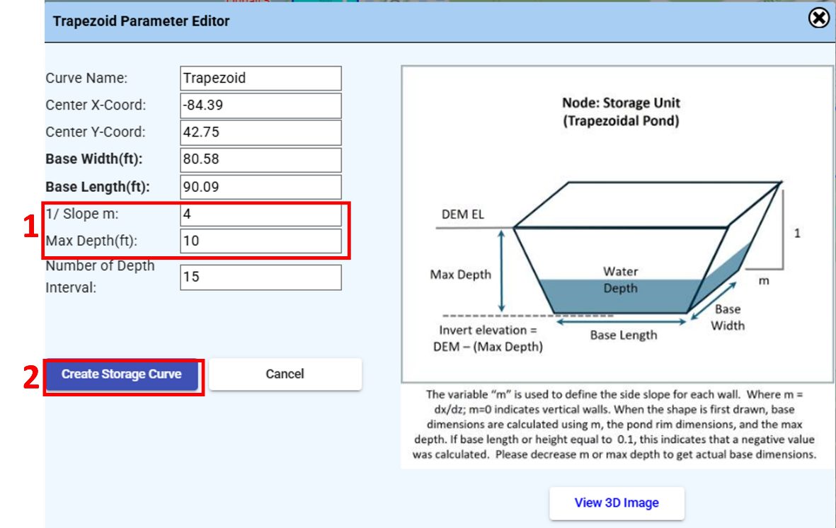
Use another single-click to add the top right corner to the map. This will complete the shape and automatically open the Trapezoidal Parameter Editor.
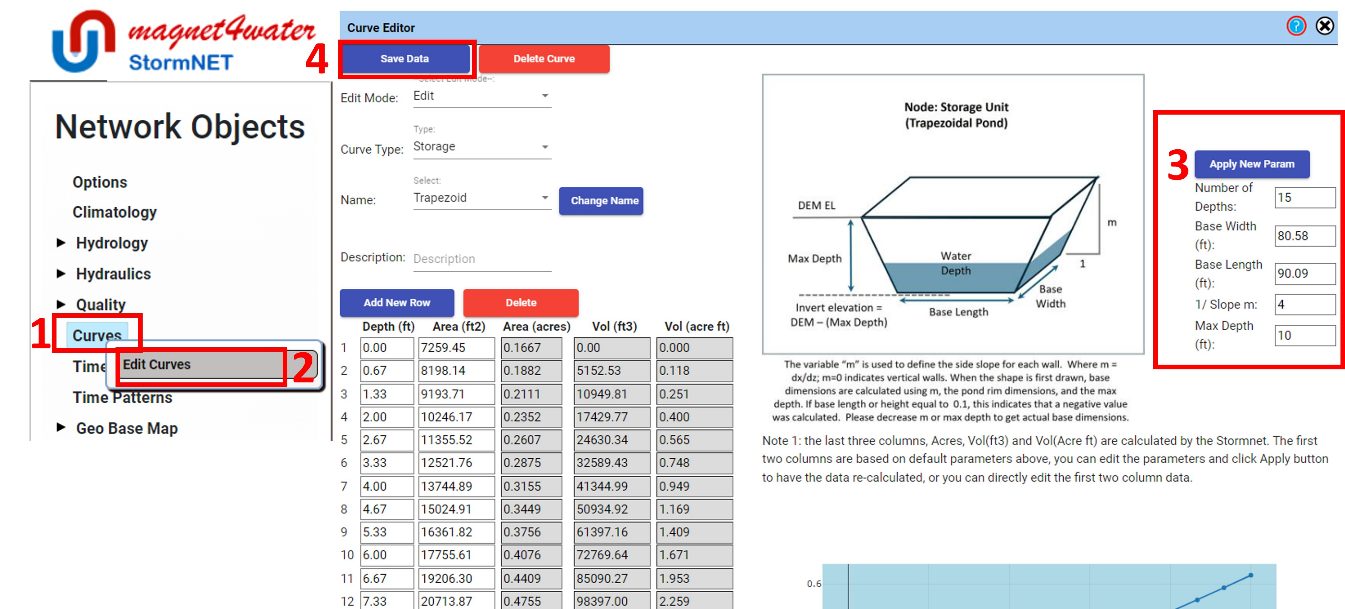
In the Trapezoid Parameter Editor window, accept defaults by clicking “Create Storage Curve”. This should automatically open the Curve Editor. Note, the drawn shape defines the lip of the trapezoidal SU, and base width and length are calculated from the drawn shape, the slope, and the max depth. If the base width and/or length are 0.01, this indicates ‘m’ or the ‘max depth’ needs to be reduced.
In the Curve Editor window, accept defaults by clicking “Save Data” (to manually open the curve editor: Curves (click, right click) > Edit Curves).
(For “Custom/Tabular SU”) Stop drawing storage units: Hydraulics > Nodes > Storage Unit (click, right click) > Stop Drawing (Stop drawing is automatic for other pre-defined SU types)
Link the Junction and the Storage Unit with a Conduit
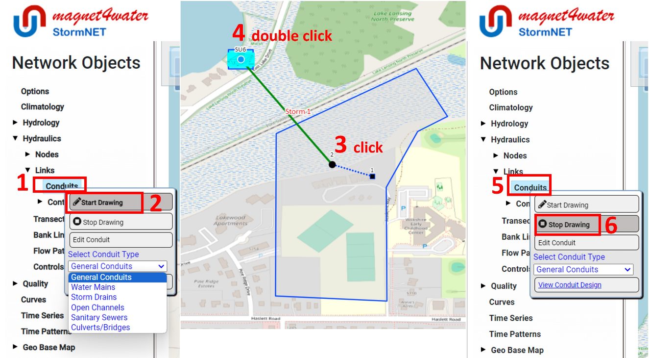
Under Network Objects: Hydraulics > Links > Conduits (click, right click) > Start Drawing
Click once on the junction to snap the conduit’s starting position to it. A blue line will extend from the node as you move the cursor.
Double click on the storage unit to snap the conduit’s ending position to it.6
Stop drawing conduits: Hydraulics > Links > Conduits (click, right click) > Stop Drawing
Add an Outfall
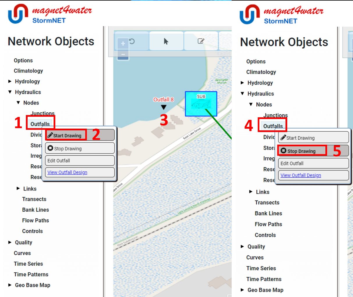
Under Network Objects: Hydraulics > Nodes > Outfalls (click, right click) > Start Drawing
Use a single-click to add the junction to a place on the map
Stop drawing outfalls: Hydraulics > Nodes > Outfalls (click, right click) > Stop Drawing
Link the Storage Unit to the Outfall with a Weir
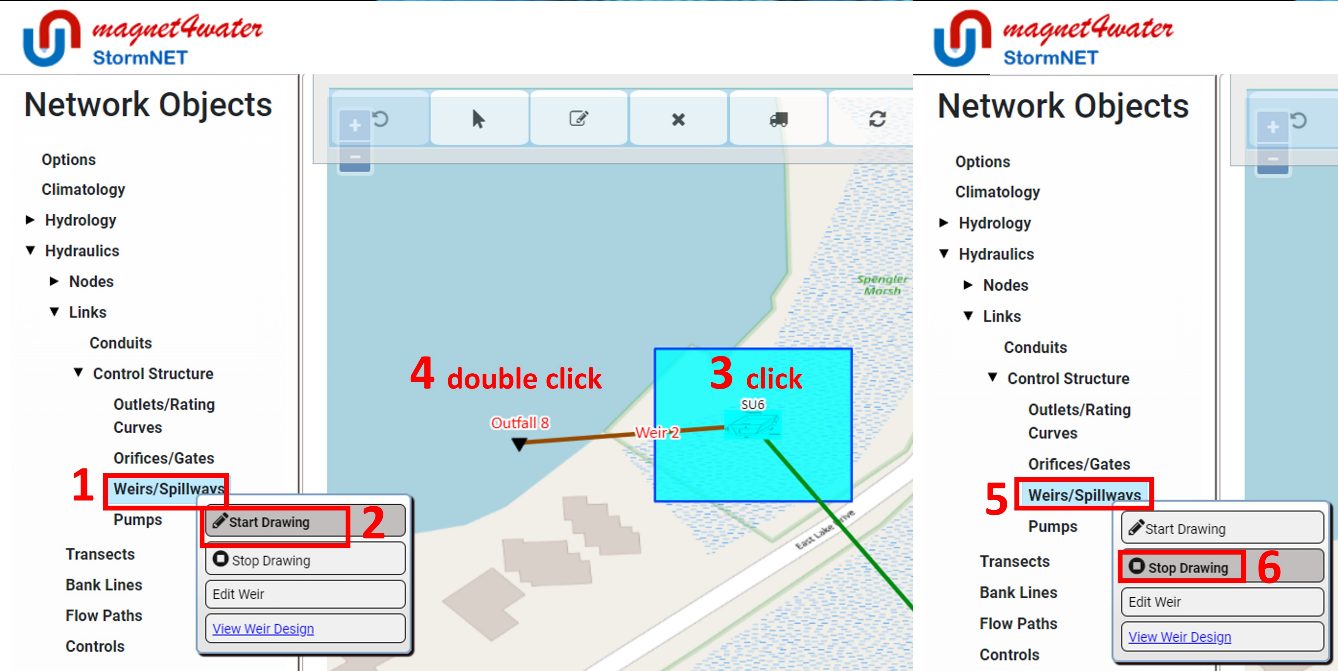
Under Network Objects: Hydraulics > Links > Control Structures > Weirs/Spillways (click, right click) > Start Drawing
Click once on the storage unit to snap the conduit’s starting position to it. A blue line will extend from the node as you move the cursor.
Double click on the outfall to snap the conduit’s ending position to it.
Stop drawing weirs: Hydraulics > Links > Control Structures > Weirs/Spillways (click, right click) > Stop Drawing
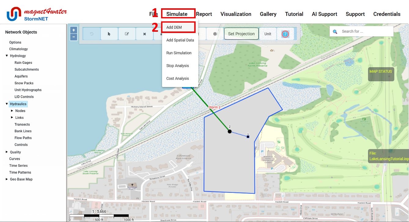
Get Object Elevations from DEM
Simulation > Add DEM
After a short while, the Invert Elevations for all Node (the junction, storage unit, and outfall) and subcatchment objects will be automatically updated based on DEM.7
(Optional) Check the elevations and offsets assigned to various objects, and modify if needed.
Modify Junction object attributes:
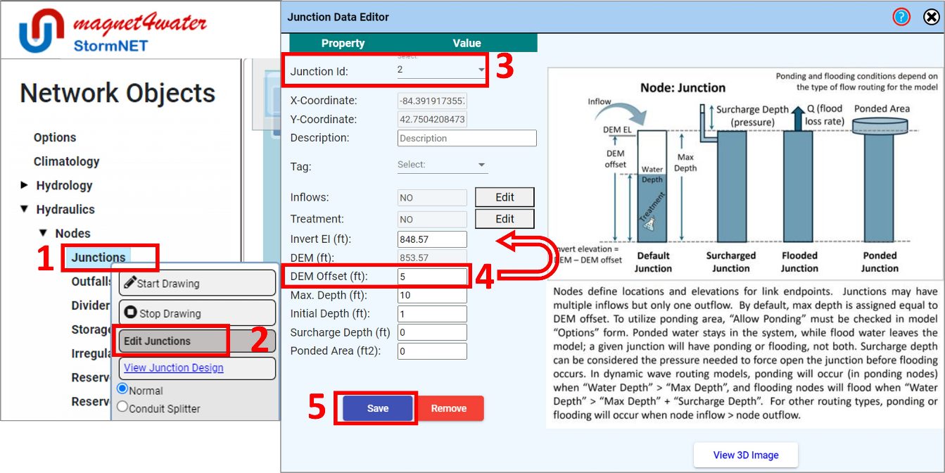
Open the Junction Editor: Under Network Objects: Hydraulics > Nodes > Junctions (click, right click) > Edit Junctions
Confirm the Junction Id is ‘2’
Edit the ‘DEM Offset’ to change the junction’s Invert Elevation (Invert Elevation = DEM – DEM Offset)
Repeat the process above to change Invert Elevations and/or other parameters for Nodes and Links.
Add a Rain Gage
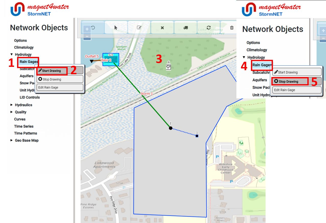
Under Network Objects: Hydrology > Rain Gages (click, right click) > Start Drawing
Use a single-click to add the rain gage to the map8
Stop drawing rain gages: Hydrology > Rain Gages (click, right click) > Stop Drawing
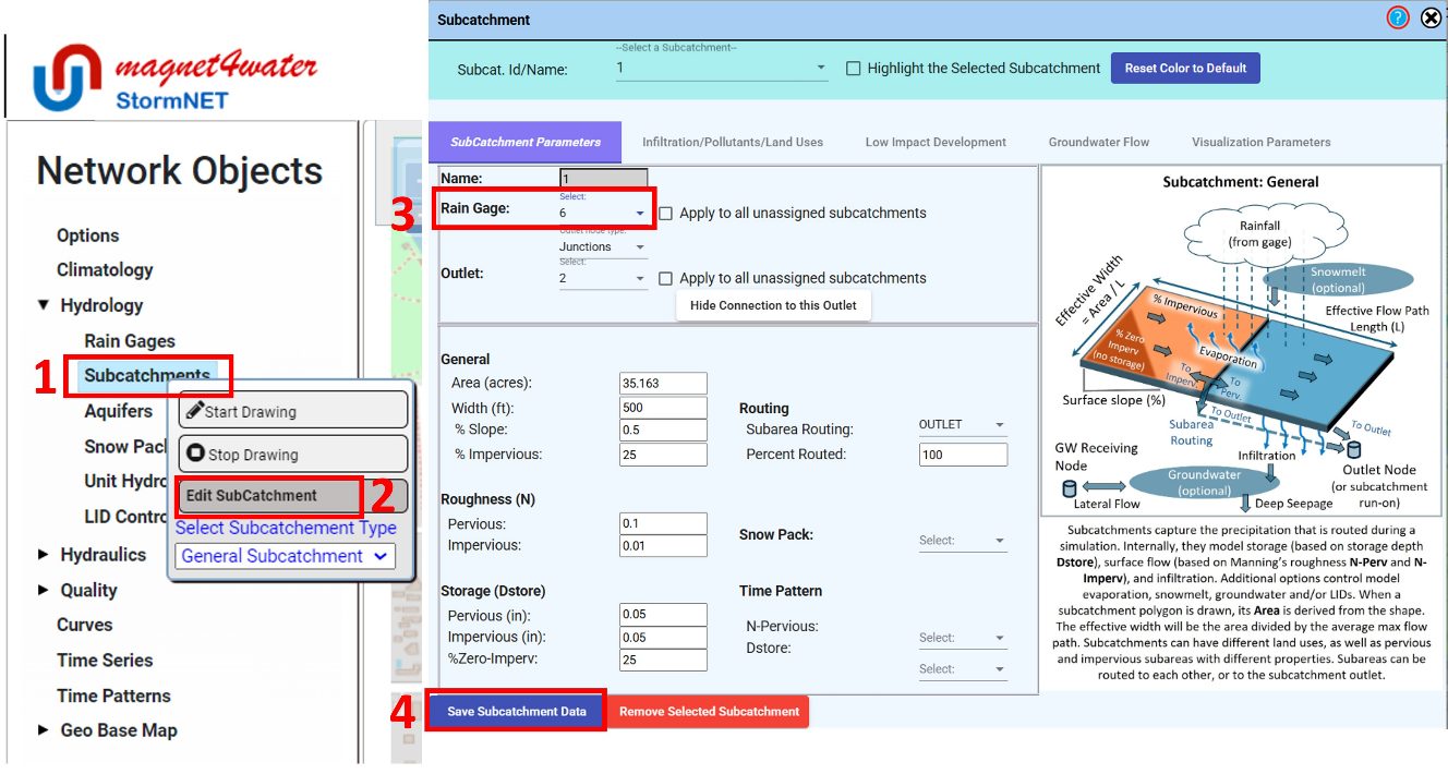
Link the Rain Gage to the Subcatchment
Open the Subcatchment Editor (see Section 5a)
Confirm Subcatchment ‘1’ is selected in Subcat. Id/Name
Select the rain gauge id (e.g. ‘6’) next to Rain Gage
Click ‘Save Subcatchment Data’ and exit the Subcatchment Editor
Define the Storm Event
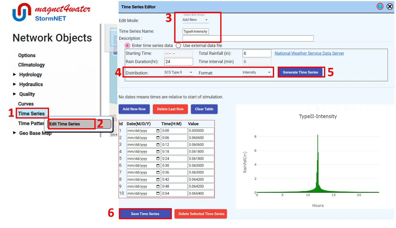
Under Network Objects: Time Series (click, right click) > Edit Time Series
Select ‘Add New’ from Edit Mode
Enter ‘TypeII-Intensity9’ in the Time Series Name.
Pick ‘SCS Type II’ for ‘Distribution’ and ‘Intensity’ for ‘Format’
Update the Rainfall Depth to reflect local conditions10
Change the ‘Rain Duration’ and/or ‘Total Rainfall’, if desired
Click ‘Generate Time Series’ to reflect changes
Click ‘Save Time Series’
Close the Time Series Editor
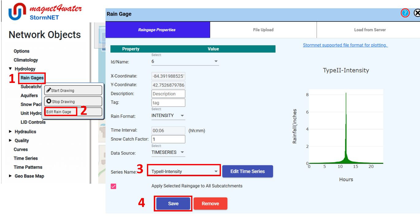
Open the Rain Gage editor:
single-click on the Rain Gage marker in the map display, OR
Hydrology > Rain Gage (click, right click) > Edit Rain Gage
Select ‘TypeII-Intensity’ as the Series Name11
Click ‘Save’ and close the Rain Gage editor.
Define Simulation Settings
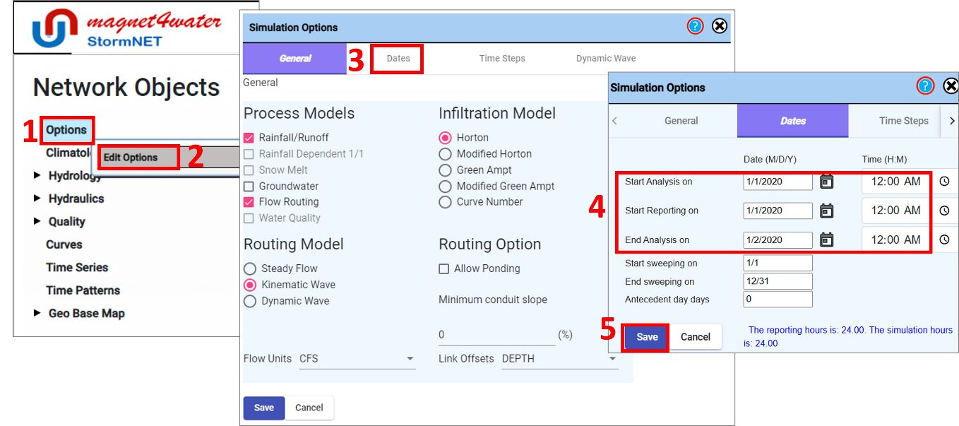
Under Network Objects: Options (click, right click) > Edit Options
Default Process Models, Infiltration Model, and Routing Model may be used.
Switch to the Dates tab
Assign the Date (M/D/Y) and Time (H:M) for Start Analysis and End Analysis such that the simulation last at least 24 hours12
Click ‘Save’
Defaults on the Time Steps and Dynamic Wave tabs may be used13.
Click ‘Save’ on any tab that is edited before closing the Simulation Options editor.
Save Model and Run Simulation
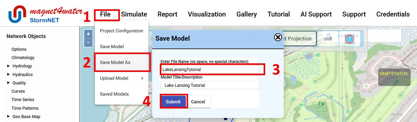
Save the changes to the model: File > Save Model As14
Enter filename and `Submit`
Submit the model for simulation:
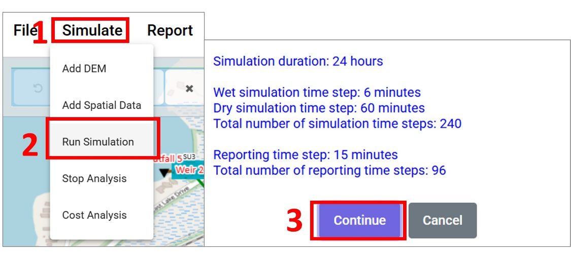
Simulate > Run Simulation
Click ‘Continue’ on the popup indicating the number of analysis and reporting steps (They should be 240 and 96 respectively).
After the model is executed, the Status Window15 will appear.
If you close the Status Window but want to examine it at a later time: Report > Simulation Status
View Plan View Results
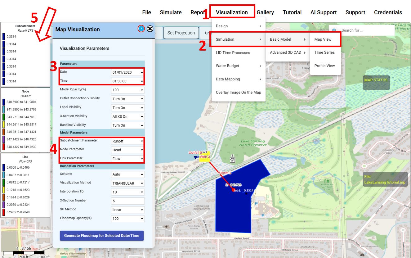
By default, plan-view results will be presented as color-coded subcatchments, links and nodes, with legends to indicate the range of values corresponding to each color16.
Use the Map Visualization Window to control the Date and Time of simulation for displaying the results, and to change parameters in subcatchment, link, and/or node.
If you close the Map Visualization Window but want to use it again: Visualization > Simulation > Basic Model > Map View
Inspect the legend and map to see model output values.
View Water Budget Plots
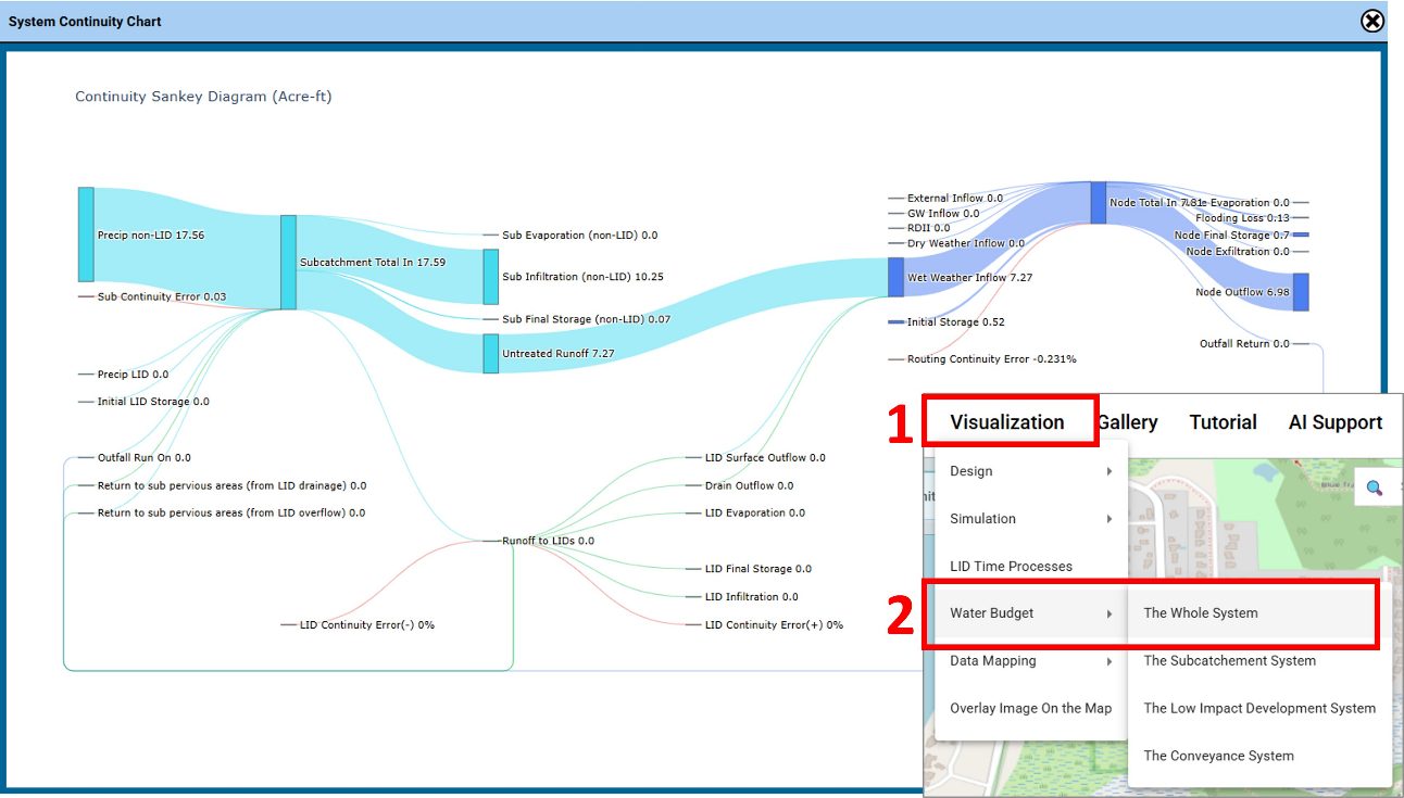
Inspect the water budget for the whole model: Visualization > Water budget > The Whole System
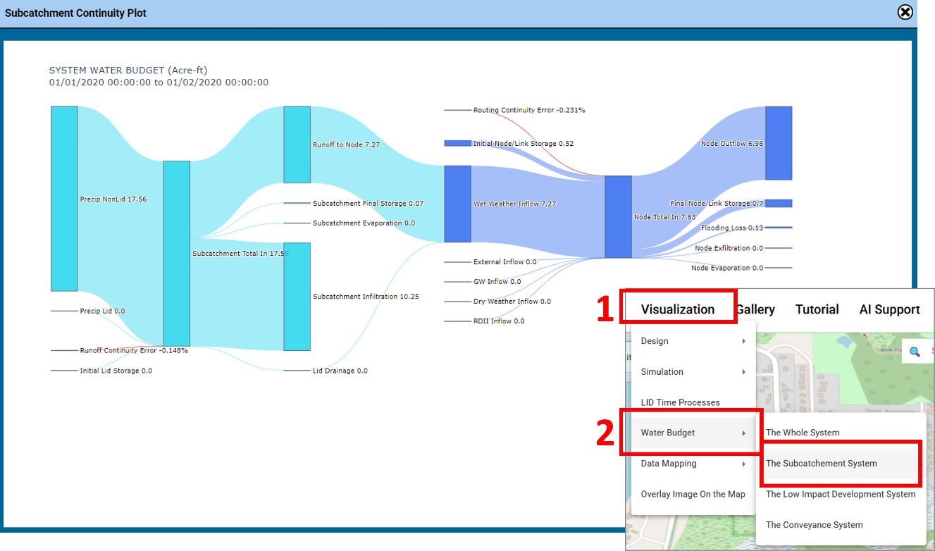
Inspect the water budget for the subcatchments: Visualization > Water budget > The Subcatchment System
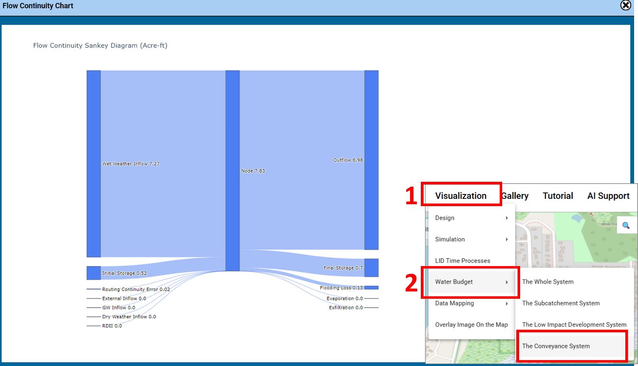
Inspect the water budget for model flow: Visualization > Water budget > The Conveyance System
View Time-series Results
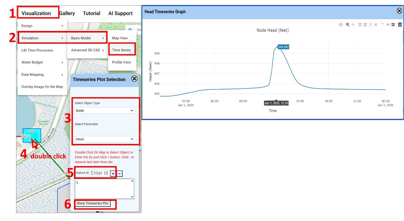
Visualization > Simulation > Basic Model > Time Series
In Timeseries Plot Selection:
Select ‘Node’ as the Object Type
Select ‘Head’ as the Parameter
Double-click on the storage unit in the map display (or enter the object ID)
Click the `+` button to add the storage unit ID to the Feature ID List
Click the ‘Show Timeseries Plot’
A plot will automatically appear showing the head results in the storage unit over the entire simulation duration.
View Results along a Profile
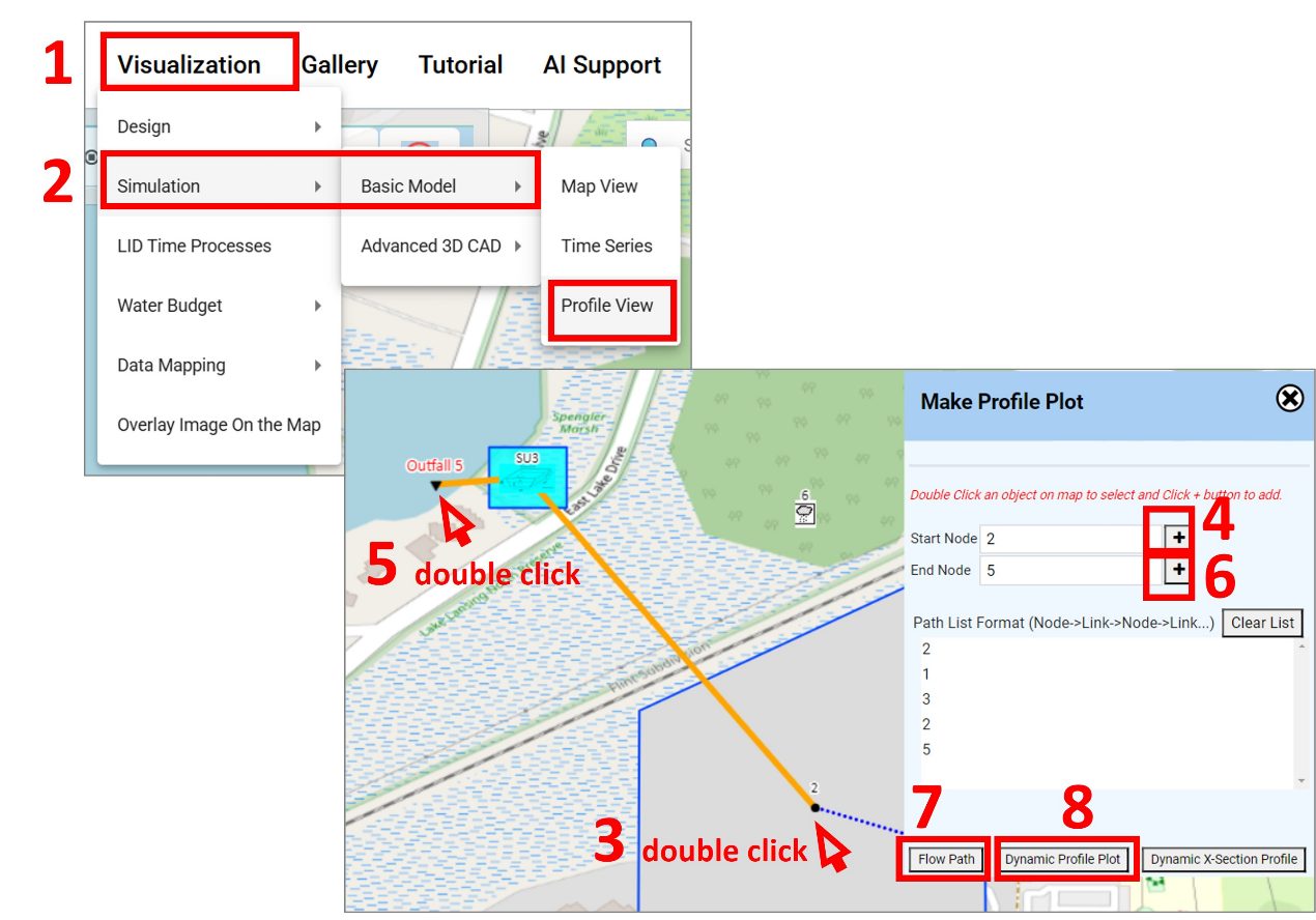
Visualization > Simulation > Basic Model > Profile View (this tool can also be used in design mode, prior to simulation, to check elevations and slopes. To access profile design mode: Visualization > Design > Profile View).
In Make Profile Plot:
Double-click on the junction in the map display
Click the + button next to Start Node to make the junction the start of the profile.
Similarly, double-click on the outfall and click the + button next to End Node to make the outfall the end of the profile.
Click the ‘Flow Path’ button to create the flow path from the Start Node to the End Node18.
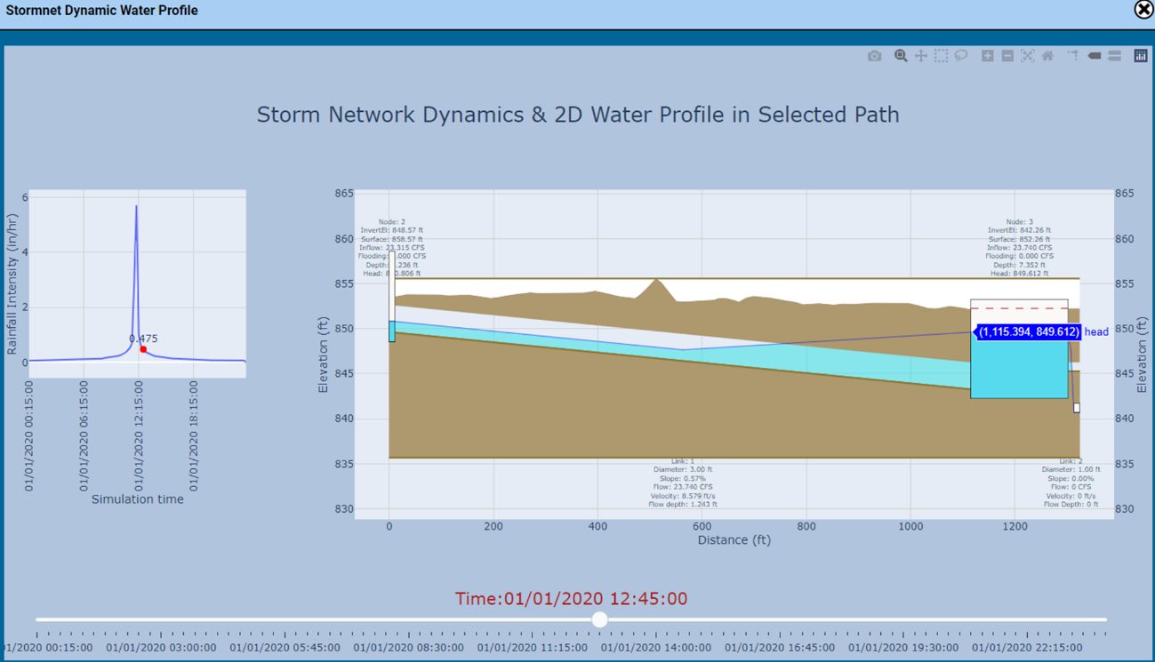
Click on the ‘Dynamic Profile’ button to launch the Dynamic Profile plot19,20
View 3D results
To display the model in 3D as it is being created/edited:
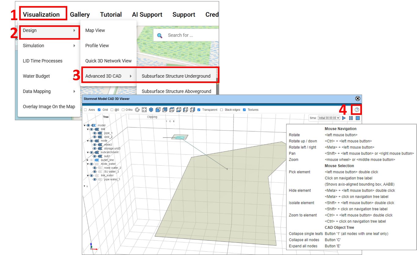
To display the most recently simulated model (and its results) in 3D
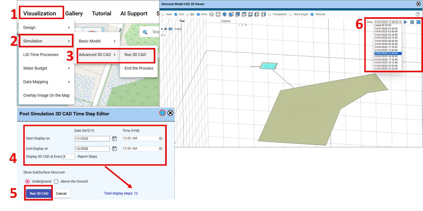
Visualization > Simulation > Advanced 3D CAD > Run 3D CAD
Set the display period start/end and display interval (e.g., every 8 report steps) and click ‘Run 3D CAD’23
After some time the simulated CAD will be displayed.
Use the controls in the top right to see water levels at various times.
Legacy 3D plot
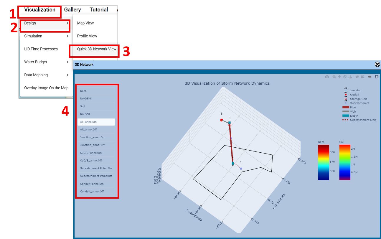
Visualization > Design > Quick 3D Network View
The mouse may be used to rotate/zoom the plot, and the left panel controls to toggle features on and off (DEM and Soil maps are available if they were extracted in step 1).
REFINING THE MODEL
Add Evaporation
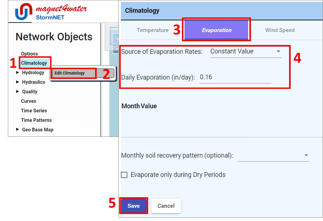
Under Network Objects: Climatology (click, right click) > Edit Climatology
Switch to the ‘Evaporation’ tab
For this short simulation, select ‘Constant’ as the Source of Evaporation Rates, and assign the Daily Evaporation (e.g. 0.16 in/day).
Click ‘Save’ and close the Climatology tab
Modify Infiltration Method
By default, the Horton method is used to estimate infiltration within subcatchments
To change the method used for all subcatchments24:
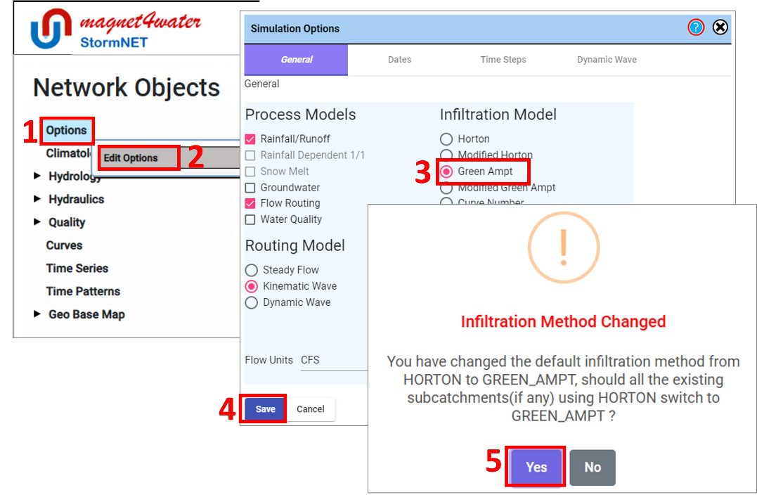
Under Network Objects: Options (click, right click) > Edit Options
Choose a different option under ‘Infiltration Model’ (e.g., Green Ampt)
Click ‘Save’
Click ‘OK’ when a popup asks to switch all existing subcatchments and close the Simulation Options editor
To assign subcatchment infiltration parameters:
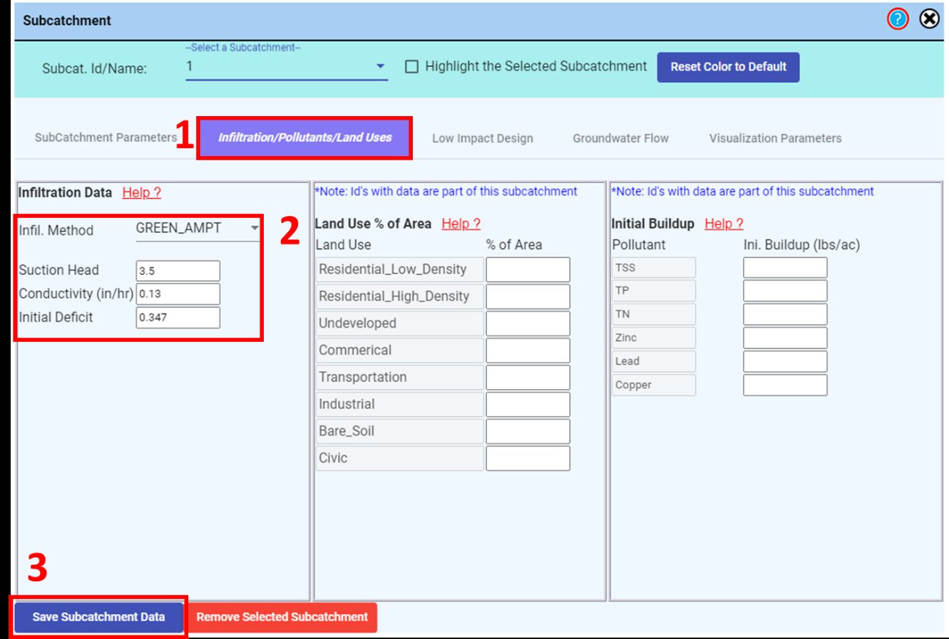
Open the Subcatchment Editor (see Section 5a)
Confirm Subcatchment ‘1’ is selected
Switch to the Infiltration / Pollutants / Land Uses tab
Under Infiltration Data section, ensure Infil. Method is ‘GREEN_AMPT’
Examine the default values and update if needed/justified
For Green Ampt: Suction head = 3.5, Conductivity = 0.13 in/hr, initial deficit = 0.347
Click ‘Save Subcatchment Data’ and close the Subcatchment editor
(Optional) Create/Edit an Aquifer
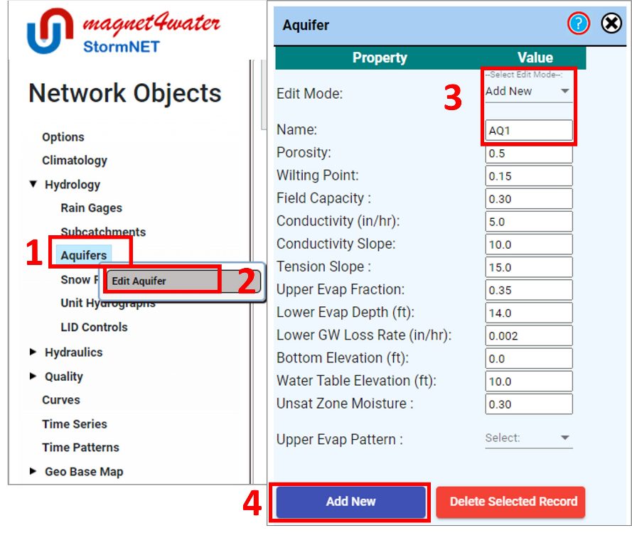
Under Network Objects: Hydrology > Aquifers (click, right click) > Edit Aquifer
Select Edit Mode ‘Add New’
When adding a new aquifer: Give the aquifer a name (e.g., AQ1; must be unique from other aquifer names). If editing an existing aquifer: Select from the dropdown (e.g., ‘Aquifer’)
Utilize the default parameter values; Bottom Elevation and Water Table Elevation will be updated in the next step.
Click ‘Add New’ or ‘Save Record’ and close the Aquifer editor.
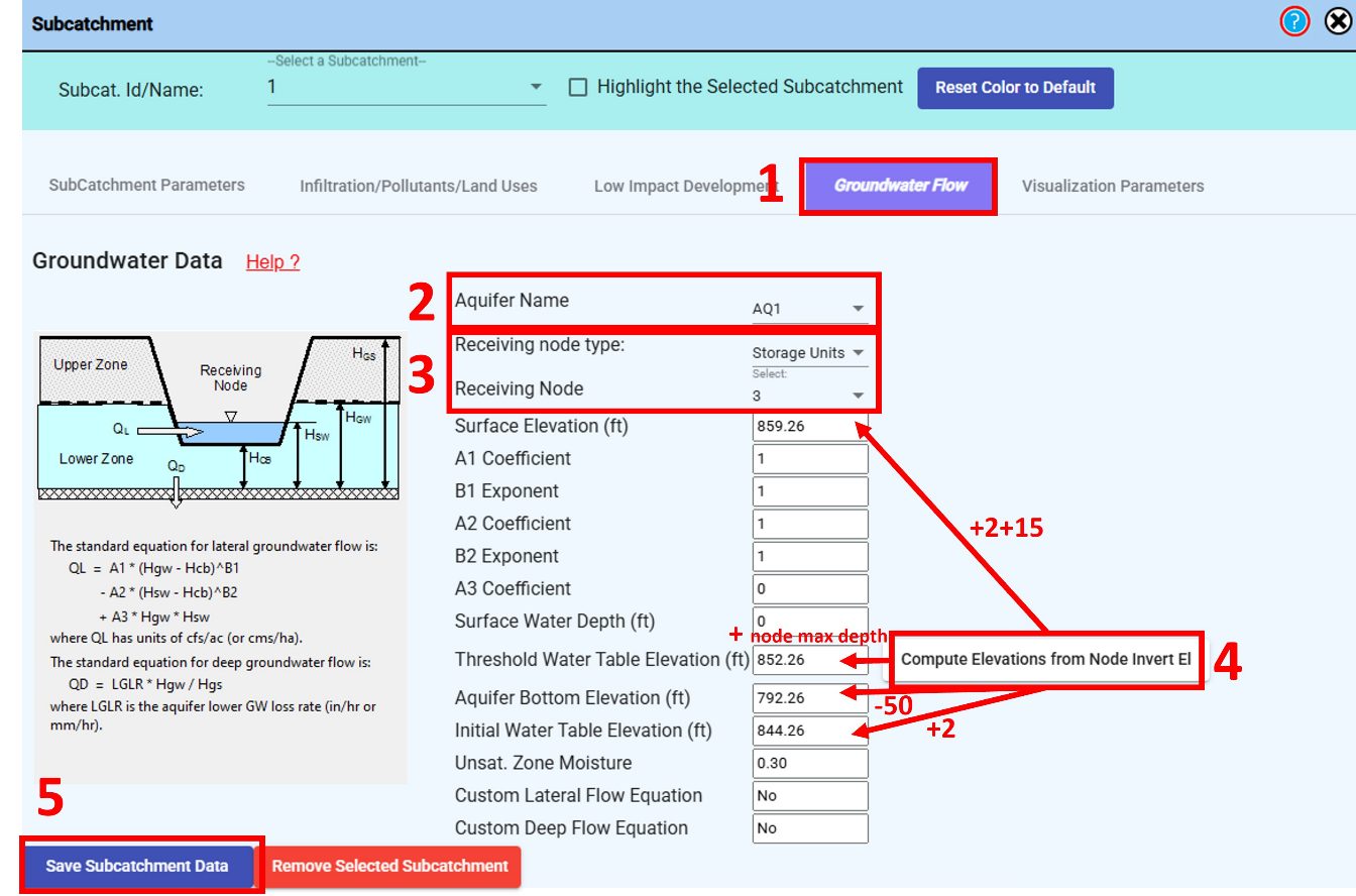
Link the Aquifer – from Subcatchment to Receiving Node
Open the Subcatchment Editor (see Section 5a)
Confirm Subcatchment ‘1’ is selected
Switch to the Groundwater Flow tab
Select the Aquifer Name (e.g., AQ1 created in the previous step)
Assign the aquifer receiving node:
Select ‘Storage Units’ as the Receiving node type
Select the storage unit, ‘3’, as the receiving node
Assign elevation parameters:
Click the ‘Compute Elevations from Node Invert El’ button to assign the values to the ‘Surface Elevation’, ‘Threshold Water Table Elevation’, ‘Aquifer Bottom Elevation’, and ‘Initial Water Table Elevation’ based in the receiving node Invert Elevation26,27.
If needed modify the ‘Surface Elevation’ and ‘Threshold Water Table Elevation’ based on the DEM contours and the Subcatchment centroid elevation.
Click ‘Save Subcatchment Data’ and close the Subcatchment editor.
(Optional) Edit/Define a Pollutant
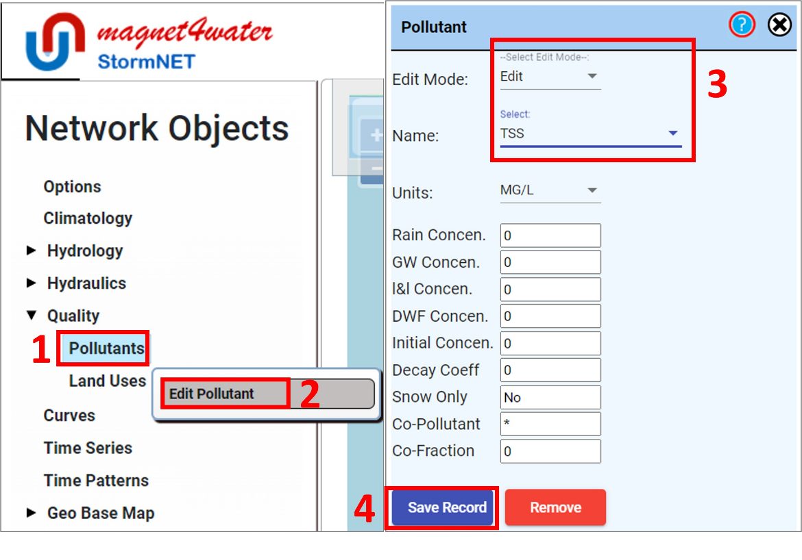
Under Network Objects: Quality > Pollutants (click, right click) > Edit Pollutants
Use Edit Mode to inspect/modify an existing pollutant by selecting ‘Edit’, or create a new pollutant by selecting ‘Add New’
If editing an existing pollutant:
Select a pollutant name (e.g., TSS)
Inspect/modify values; the pollutant loading in the subcatchment can be added to the model to a defined land use in the next step.
Click ‘Save Record’ and close the Pollutant editor.
If adding a new pollutant:
Give the Pollutant a name (e.g., TSS1; must be unique from other pollutants)
Use the default values; the pollutant loading in the subcatchment can be added to the model to a defined land use in the next step.
Click ‘Add New’ and close the Pollutant editor.
(Optional) Edit/Define a Land Use
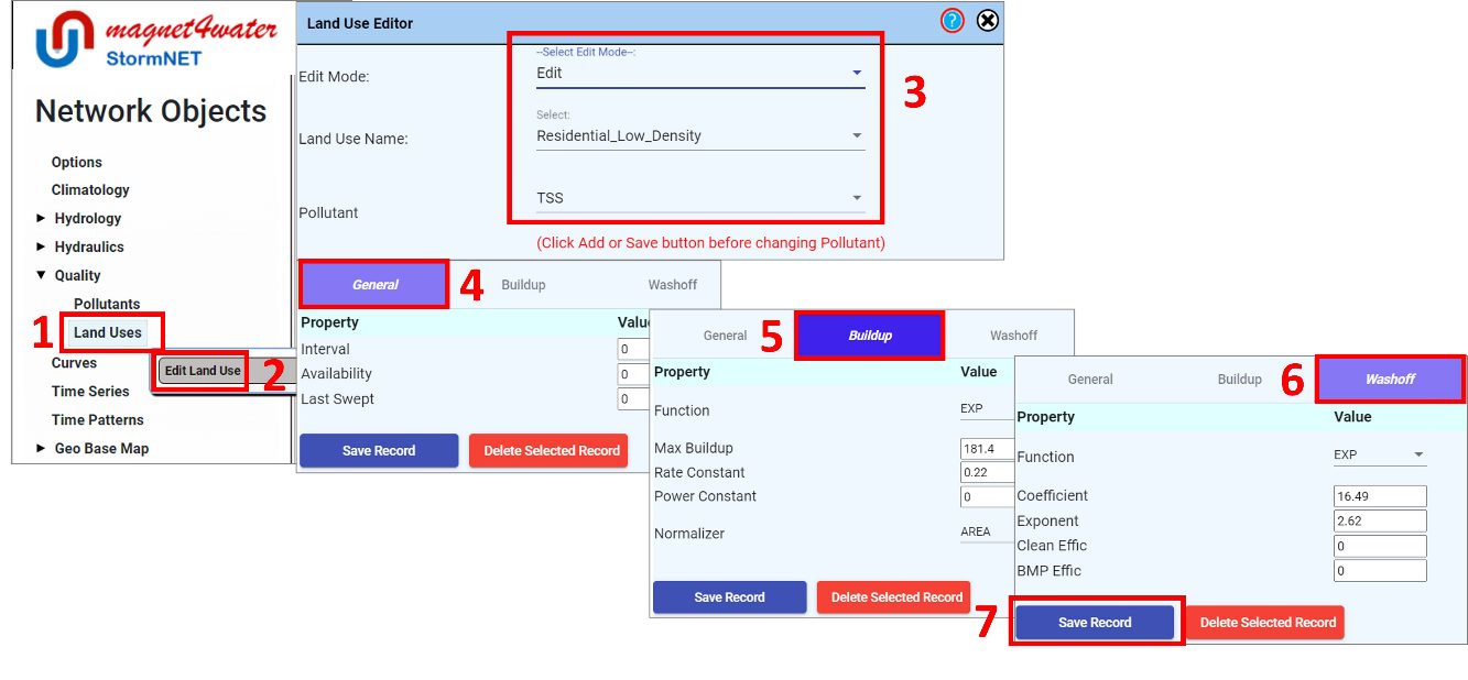
Under Network Objects: Quality > Land Uses (click, right click) > Edit Land Use
Use Edit Mode to inspect/modify an existing land use by selecting ‘Edit’, or create a new land use by selecting ‘Add New’
If editing an existing land use: Select a land use name (e.g., ‘Residential_Low_Density’)
If adding a new land use: Give the land use a name (e.g., Residential; must be unique from other land use names)
Select the Pollutant edited/created in the previous step (e.g., ‘TSS’)
Inspect/edit the default parameters on the General tab
Switch to the Buildup tab and inspect/edit the default parameters
Switch to the Washoff tab and inspect/edit the default parameters
Click ‘Save Record’ or ‘Add New’ and close the Land Use editor
Link Land Use to the Subcatchment
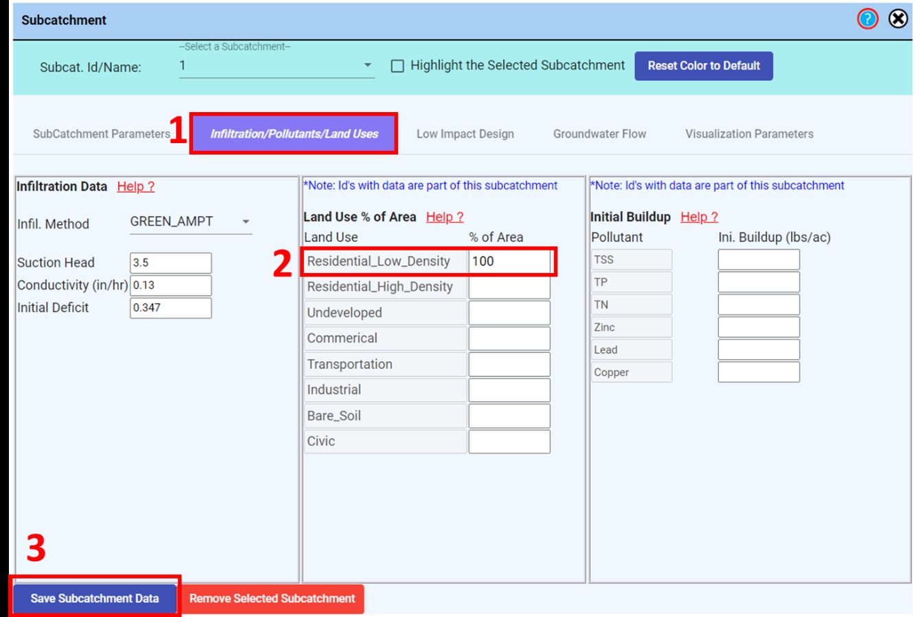
Open the Subcatchment Editor (see Section 5a)
Confirm Subcatchment ‘1’ is selected
Switch to the Infiltration/Pollutants/Land Uses tab
Under Land Use % of Area, enter 100 next to a land use type (e.g., ‘Residential_Low_Density’ or another land use edited/created in the last step)30
(Optional) Edit/Create a LID Control
Under Network Objects: LID Controls (click, right click) > Edit LID Control
Use Edit Mode to inspect/modify an existing LID Control by selecting ‘Edit’, or create a new LID by selecting ‘Add New’
If editing an existing LID:
Select an LID name (e.g., ‘GreenRoof)
Inspect/edit values (note, there are multiple tabs depending on the Lid Type)
If adding a new LID:
Give the LID a name (e.g., Roof; must be unique from other LID names)
Select a Lid Type (e.g., Green Roof)
Use default values (note there are multiple tabs depending on the Lid Type)
Click ‘Save’ and close the LID Control Editor
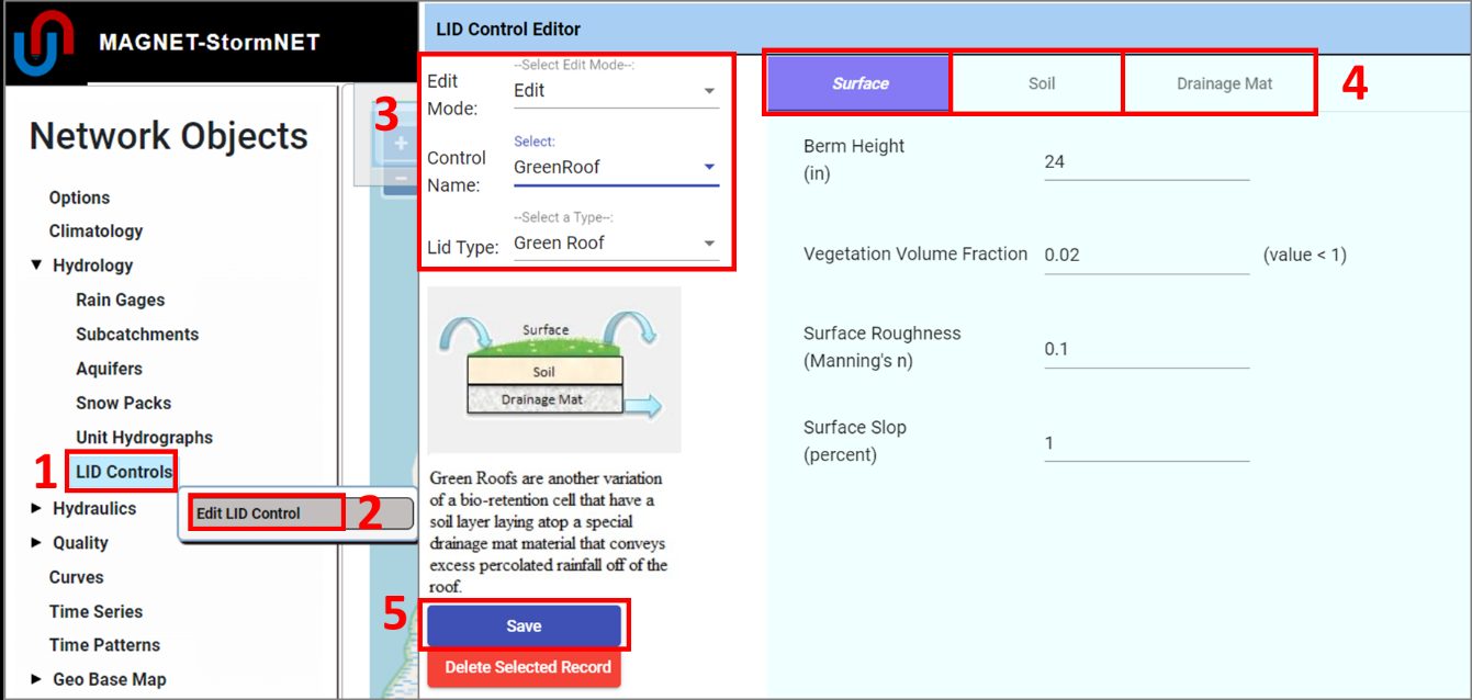
Create Green Roof Subcatchment
Create subcatchment over building footprint (see Section 3)
Select ‘Green Roof(LID)’ as the Subcatchment Type, before clicking ‘Start Drawing’. This will automatically assign the GreenRoof LID to the subcatchment.
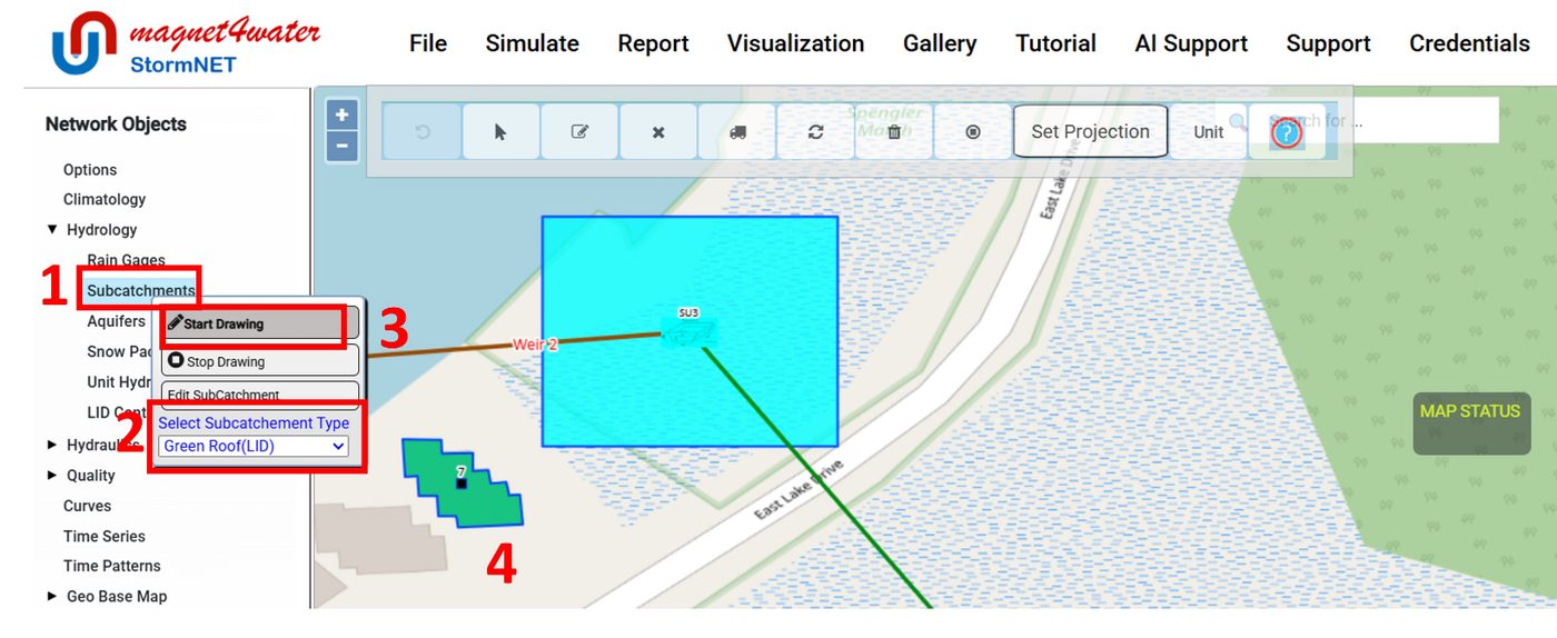
Link subcatchment to rain gauge 6 and storage unit 3 (see Sections 5 & 12)
AddDEM to subcatchment vertices (see Section 10)
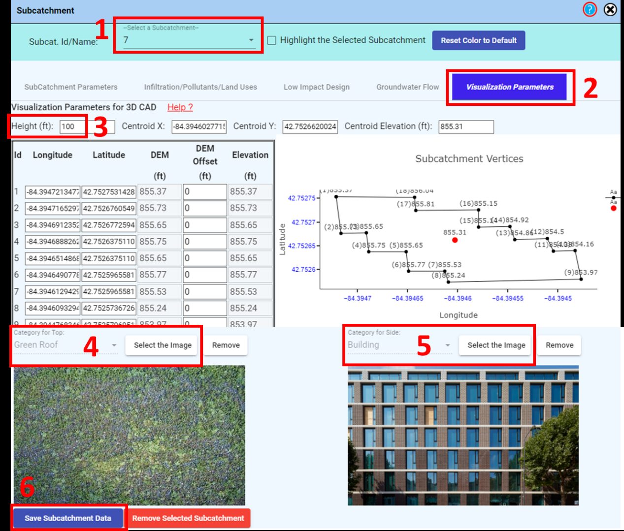
Set Building Visualization
Open the Subcatchment Editor (see Section 5a)
Confirm Subcatchment ‘7’ is selected
Switch to Visualization Parameters tab
Inspect/edit the Building height (e.g. 100 feet)
(Optional) edit the Top and Side Textures using the ‘Select the Image’ buttons.
Green Roof subcatchment Top default is Green Roof > Green Roof 11.
Green Roof subcatchment Side default is Building > Building 98.
Click ‘Save Subcatchment Data’ and close the Subcatchment Editor
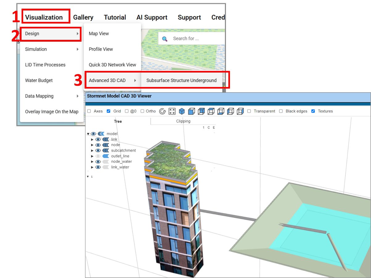
View the 3D representation of the Green Roof just created (see Section 20a).
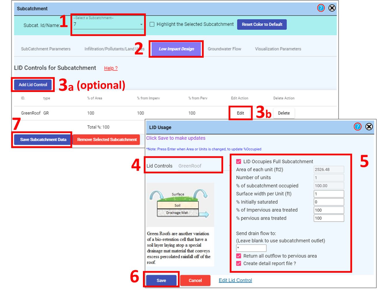
Edit/Link the LID Control to the Subcatchment
Open the Subcatchment Editor (see Section 5a)
Confirm Subcatchment ‘7’ (the newly created LID) is selected
Switch to the Low Impact Development tab
(Optional) To add a new LID Control to the subcatchment:
Click ‘Add Lid Control’, this will open the LID Usage editor.
In LID Usage editor:
Select an LID (e.g., ‘Roof’ if created in the previous step [see Section 28])
Check the ‘LID Occupies Full Subcatchment’32 box, or enter the Area of each unit and Number of units to have the LID occupy only a portion of the Subcatchment (% of subcatchment occupied is updated automatically).
Check the ‘Create detail report file’ (this is required to display LID processes after simulation).
To edit an existing LID Control (‘GreenRoof’ should already be added, as it was selected as the subcatchment type before drawing):
Click ‘Edit’, this will open the LID Usage editor
Inspect/edit the area, and other options. Check the ‘Create detail report file’ (this is required to display LID processes after simulation).
Click ‘Save’ and close the LID Usage Editor
If a new LID Control was added, it should appear in the list on the Subcatchment Editor.
Click ‘Save Subcatchment Data’ and close the Subcatchment Editor
Save Model, Re-Run Simulation, and View Results
Save and run the refined model (See Section 15)
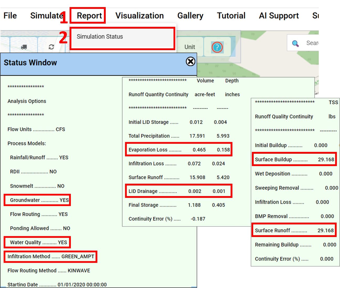
Confirm that the simulation report includes the model refinements:
Analysis Options for ‘Ground Water’ and ‘Water Quality’, and ‘GREEN_AMPT’ is used for Infiltration.
Evaporation and LID drainage are non-zero
Selected pollutant runoff is calculated.
Inspect the Low Impact Development Plots:
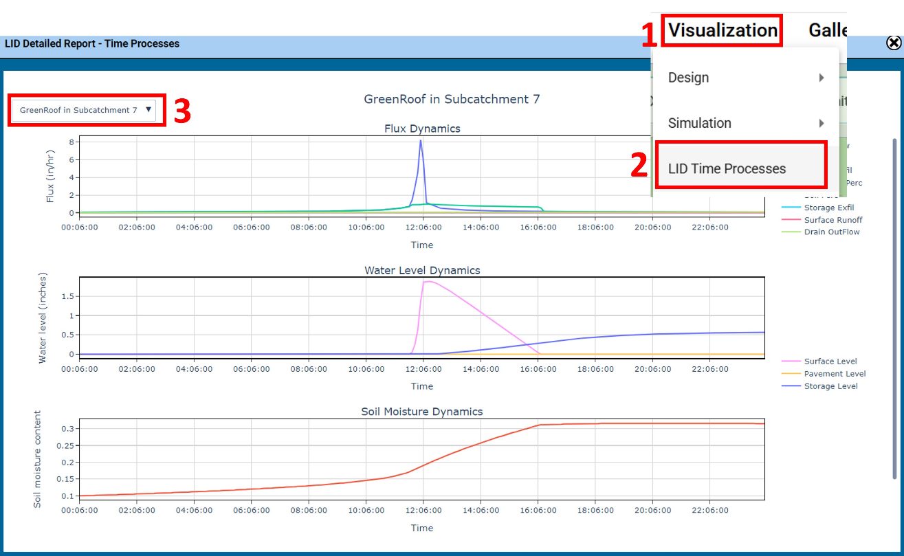
Generate the plots: Visualization > LID Time Processes (If a warning occurs, confirm that a LID has been correctly linked to a subcatchment, and that the box ‘Create detail report file’ in the LID Usage editor is checked; see Section 30e).
Select the LID linked to the model in Section 30 (e.g., ‘Greenroof in Subcatchment 7’).
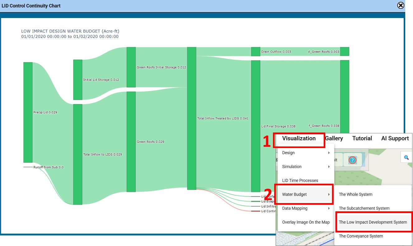
Inspect the water budget for the LID controls: Visualization > Water budget > The Low Impact Development System
Explore additional plots and results (see Sections 16 – 20)