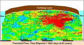
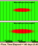
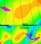
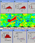
This library provides a collection of MAGNET videos, focusing on illustrating and visualizing the complex effects of heterogeneity on groundwater flow and solute transport. The library is divided into the following categories: 1) real world heterogeneity, 2) random field representation, 3) effect of spatial heterogeneity, 4) effect of coupled physical and chemical heterogeneity, 5) effect of temporal variability, 6) effect of multiscale heterogeneity, 7) macrodispersion model, and 8) monte carlo simulations.
Click the image below to view the videos.
Click here to go to Education Videos
Click the image below to view the videos.
Click here to go to Education Videos
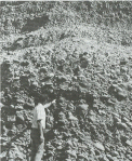
- The subsurface environment is inherently heterogeneous, exhibiting dramatic variations over surprisingly small distances. Since it is practically impossible to measure these detailed point to point variations, heterogeneity translates into uncertainty. A random field representation characterized by statistics such as mean, variance, and covariance derived from data provides a systematic way to describe the heterogeneous aquifer properties.
- Small-scale heterogeneity in conductivity causes large scale spreading of plume resulting in numerous fingers and tails. Even though ln K distribution in the field is Gaussian, the variation of plume concentration with time at any point is non-Gaussian.
- When a heterogeneous conductivity field is coupled with a heterogeneous porosity field, the effect on plume spreading is not drastic. Since porosity varies over a small range of values compared to conductivity, the impact on velocity variability is minimal. When n and K are positively/negatively correlated, the plume is slightly smaller/larger compared to when n and K are not correlated.
- When a heterogeneous conductivity field is coupled with partitioning coefficient, the effect on plume spreading is drastic. Since partitioning coefficient variability is comparable to that of conductivity, the impact on velocity variability is significant. When Kdand K are positively/negatively correlated, the plume is significantly smaller/larger compared to when Kdand K are not correlated.
- Depending on the scale of the heterogeneity with respect to the initial size of the plume, the type of plume transport is significantly different. Usually, when the plume is larger than the scale of heterogeneity, plume spreading is considerably higher. However, when the plume is much smaller than the scale of heterogeneity, the plume travels predominantly along preferential channels, while not spreading by a great extent. When the plume is extremely small compared to the scale of heterogeneity, the plume undergoes “negative transverse dispersion.”
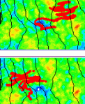
- Temporal variability caused by seasonal fluctuations, in the absence of spatial heterogeneity, causes to and fro motion of the plume, which is reversible. Generally, the plume does not undergo extensive spreading. When temporal variability interacts with spatial heterogeneity, the effect on plume transport is drastic as the plume is shred into fingers and tails. In addition, the process cannot be reversed because the plume may get trapped in a low conductivity zone, which causes enhanced spreading of the plume. When additional heterogeneities, such as partitioning coefficient, are coupled together with temporal variability and spatial heterogeneity, the effect on plume spreading is compounded.
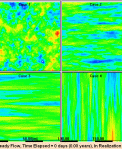
- Heterogeneity in the real world is practically not deterministic. In order to model this highly complex variable conductivity field, a stochastic approach is used. In this approach, the aquifer structure is represented using a set of statistical parameters, such as mean, correlation scales, and variance. These statistical parameters are obtained by analysis of the data.
- Mean is the geometric mean of the data, which represents the average conditions that exist in the aquifer
- Correlation scales are a measure of the spatial distance across which the aquifer properties are supposed to be correlated. This parameter can be different in all three directions making the aquifer anisotropic. However, in most cases, the horizontal correlation scales ( λxand λy) are assumed to be constant.
- Variance is a measure of how variable the aquifer properties are with respect to the mean. A higher variance means higher variability of aquifer properties and vice versa.
- Macrodispersion models predict the mean plume spreading and the overall extent of the plume. However, these models do not provide information on the maximum concentration, concentration variance and the degree of dilution.
- Multiple scales of heterogeneity have a significant impact on plume spreading. Large scales of heterogeneity provide only a “trend” for plume transport, while the smaller scales spread the plume. If the smaller scales are not modeled, the spreading of the plume is significantly less. When the smaller scales are modeled using an effective macrodispersion model the model is able to predict the overall extent of the plume. However, this model does not provide information on the maximum concentration, concentration variance and the degree of dilution.
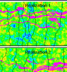
- Stochastic methods such as Monte-Carlo simulations provide information on the mean plume behavior by statistically analyzing the plume characteristics obtained from an infinite number of realizations. Monte-Carlo simulations can also provide information on the probability distribution function (PDF) of any parameter of interest, such as head, ln K , concentration at a monitoring well, and seepage and solute flux across a cross-section of the aquifer.
- Although a Gaussian distribution of ln K characterizes the random field, the concentration PDF and solute flux PDF are strongly skewed. However, the head and seepage flux PDF across a cross-section are predominantly Gaussian. In the vicinity of stresses such as pumping wells, head and seepage flux PDF may not be Gaussian.
- If the concentration PDF is assumed to be Gaussian, a mean and variance will be sufficient to estimate the probability distribution. Since concentration PDF is strongly skewed, characterizing the uncertainty is difficult. If the concentration PDF is lognormal, it can be characterized using a mean and a variance. However, concentration is strongly location dependent, and a lognormal distribution does not hold good always. Therefore, variance is not a good measure of uncertainty for concentration PDF. Hence, the actual concentration PDF is needed to determine the variability at each point of interest.
