1Introduction & Account Setup
Overview, accessing ConduitNET, creating your MAGNET4WATER account.
Browse to: https://www.magnet4water.org/conduitnet
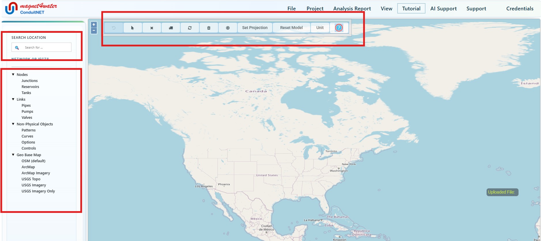
This site hosts the complete, integrated pipe network modeling, analysis, and visualization platform. The default interface environment is shown here.
Create an account: [Menu Bar] Credentials > Log In
Create an account: [Menu Bar] Credentials > Log In
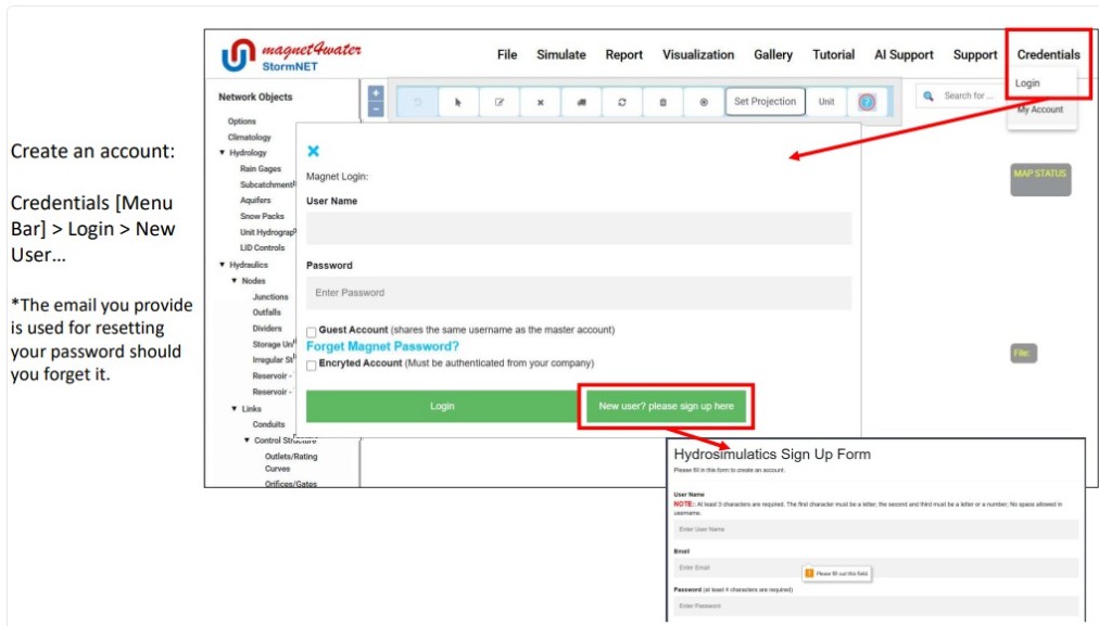
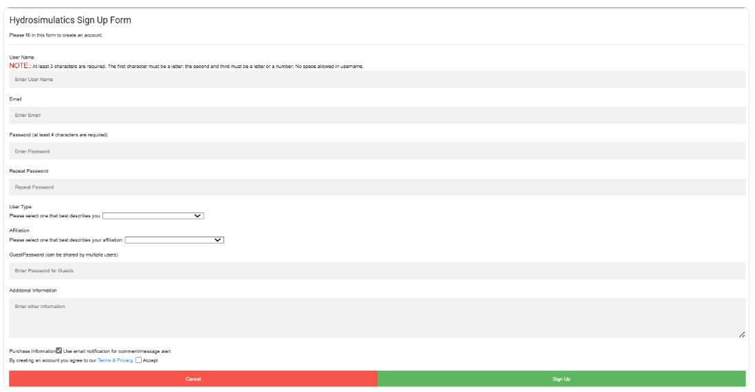
Create New Account: [Menu Bar] Credential > Log In > Sign Up)
You only need to create one account to access all the MAGNET4WATER Platforms (IGW-NET, StormNET, SwaNET ConduitNET and DataNET)
2Start a New Synthetic Project
Create a synthetic (non-geo-referenced) model — a "numerical sandbox" with no real-world map base.
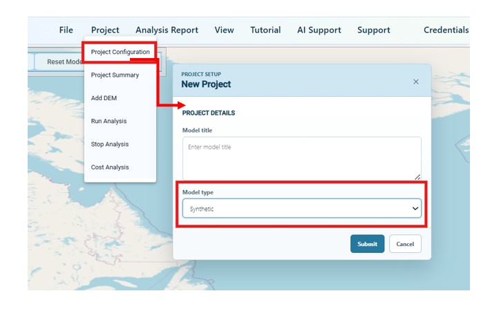
Start a New Project: [Menu Bar] Project > New Project
Use Project menu to start a new project, save the model file, upload an existing model, and view saved model INP (input) files. For this tutorial, choose the Synthetic Model Type and click Submit. This will remove the background map from the display / Working Environment so the user can work within a “numerical sandbox”. Note: By default, ConduitNET models are map-based (or geo-referenced to real-world locations). In these types of models, pipe lengths can be auto-calculated and pipe elevations can be based on a Digital Elevation Model (DEM). A Quick Tutorial for GeoReferenced models is coming soon.
3Add Nodes: Reservoir, Junctions, Tank
Add and configure the network nodes — reservoir as source, junctions as demand points, tank as storage.
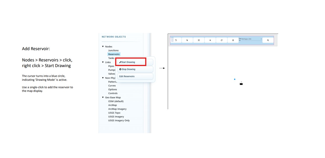
Add Reservoir: Nodes > Reservoirs > click, right click > Start Drawing
The cursor turns into a blue circle, indicating ‘Drawing Mode’ is active. Use a single-click to add the reservoir to the map display. *Note that if you hover the cursor over a node or link object, the Map Status hover field will indicate the node / link ID of that object.
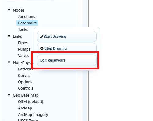
Edit Reservoir: 1. Nodes > Reservoirs > click, right click > Stop Drawing 2. Nodes > Reservoirs > click, right click > Edit Reservoirs* *A single-click on any map object also launches its Editor menu.
Select the reservoir by its Reservoir ID (1 for this example). The total head in Reservoir 1 should be set to 700ft. DEM and DEM Offset are set to zero for synthetic model. Click ‘Save’ to finalize changes before exiting the Reservoir Data Editor (‘X’ button).
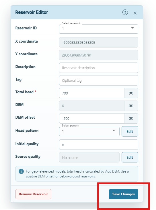
Add Junctions: Nodes > Junctions > click, right click > Start Drawing
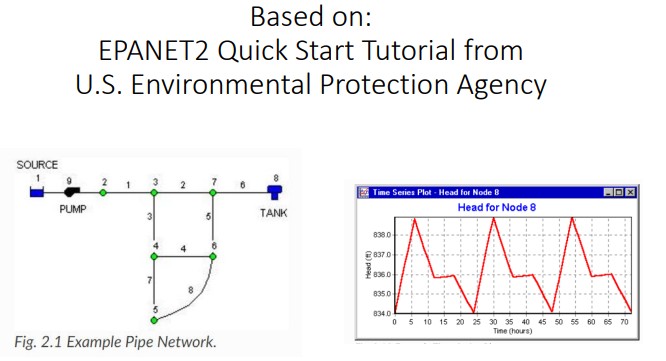
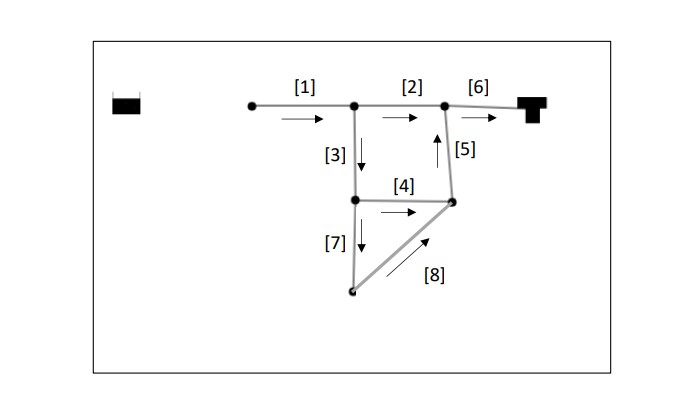
Again, the cursor turns into a blue circle, indicating ‘Drawing Mode’ is active. Use a single-click to add the six junctions to the map display. Add the notes in the approximate locations indicated in the figure. Follow the correct order so that the Junction ID matches the network plan shown here and in slide 2*. *Note that, in principle, the IDs can be different from those used in the network plan, but it makes trickier to assign junction-specific attributes from the example.
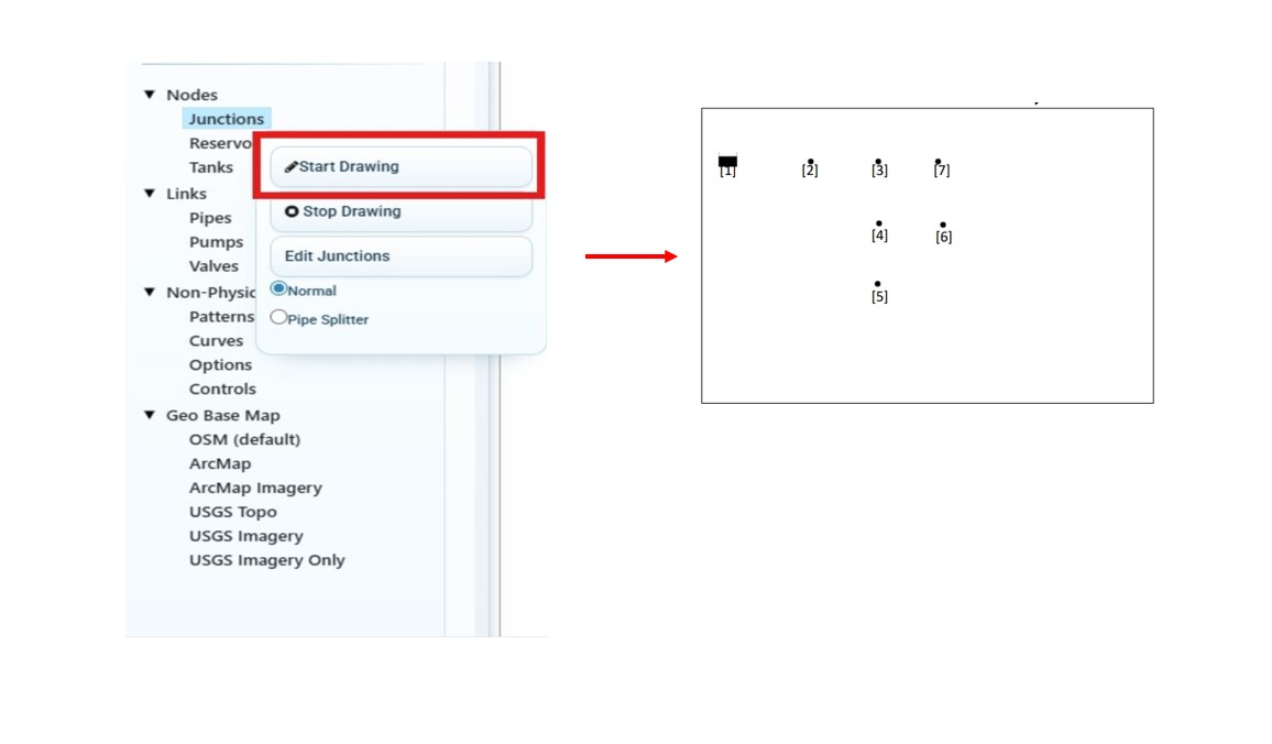
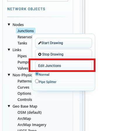
Edit Junctions: 1. Nodes > Junctions > click, right click > Stop Drawing 2. Nodes > Junctions > click, right click > Edit Junctions
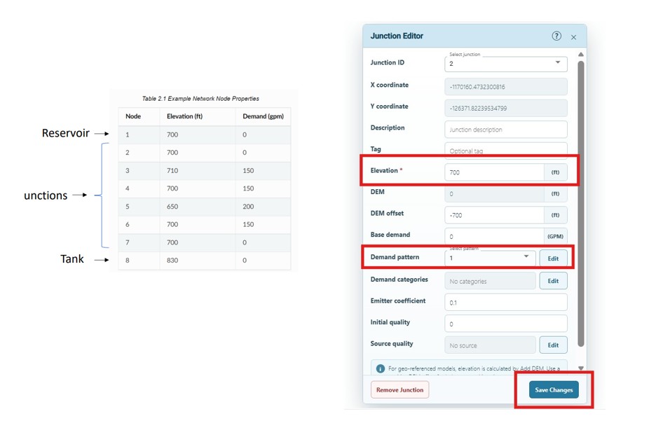
Edit Junctions (cont.): Reservoir Junctions Tank
Select the different junctions by their Junction ID (2-7 for this example) for attribute editing. The total head in Junction 2 should be set to 700ft. The Base Demand should be set to zero. Click ‘Save’ to finalize changes before selecting a new junction for editing: Junction 3, edit attributes, Save; Junction 4, edit, Save; and so on… After updating and saving all of the junctions, close the Junction Data Editor window (‘X’ button).
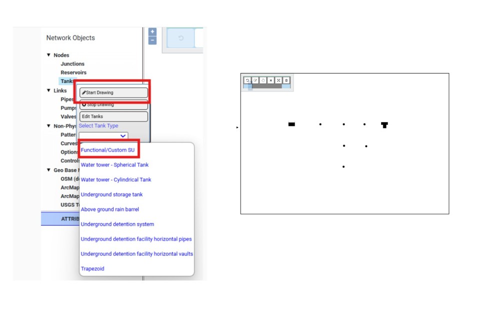
Add Tank: Nodes > Tanks > click, right click > Start Drawing
The cursor turns into a blue circle, indicating ‘Drawing Mode’ is active. 1. From the dropdown box, select Functional/Custom SU, 2. Click Start Drawing button and use a singleclick to add the tank to the map display.
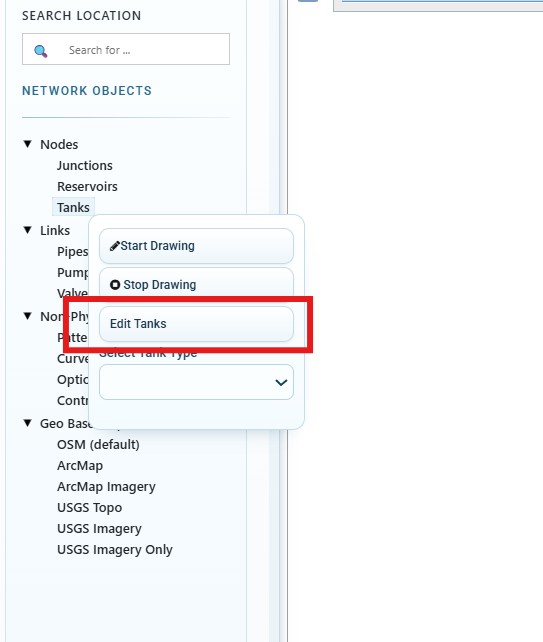
Edit Tank: 1. Nodes > Tanks > click, right click > Stop Drawing 2. Nodes > Tanks > click, right click > Edit Tanks
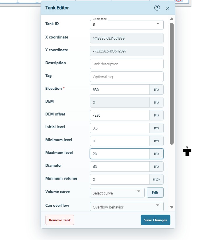
Select the tank using the Tank ID (8 for this example). Assign a elevation of 830ft. Assign an initial water level of 3.5ft. Assign a minimum level of 0ft. Assign a maximum level of 20ft. Assign a diameter of 60ft. Click ‘Save’ to finalize the changes before closing the Tank Data Editor.
4Add Pipes & Pumps (Links)
Draw pipes connecting your nodes, define a pump curve, and add pumps to lift water into the tank.
Add Pipes: Links > Pipes > click, right click > Start Drawing
Again, the cursor turns into a blue circle, indicating ‘Drawing Mode’ is active. Click once on Junction 2 to snap the pipe’s starting position to it. A blue line will extend from the node as you move the cursor. Double click on Junction 3 to snap the pipe’s ending position to it or right click on Junction 3 and select 'End Drawing'. *Once a pipe is started (linked to the starting node), a single click only places a vertex for drawing purposes. The pipe is still “open” (not snapped to an end node). *A pipe must have a starting and ending node. “Bad” pipes are deleted from the map display. If you get a thin blue line this indicates the link was unsuccessful. When this happens click “Undo” on the map toolbar, or “Stop Drawing” and “Start Drawing” on the Link menu.

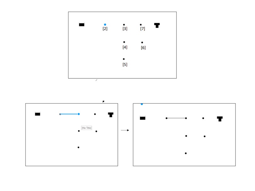
Continue adding pipes to the network in the order indicated here and on slide 2. *Do not use a pipe to link the reservoir to Junction 2. A pump will be used as a link between the reservoir and Junction 2.
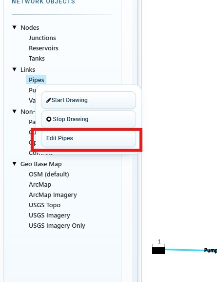
Edit Pipes: 1. Links > Pipes > click, right click > Stop Drawing 2. Links > Pipes > click, right click > Edit Pipes
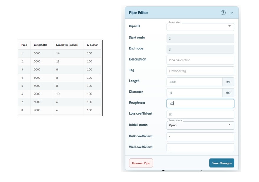
Select the different pipes by their Pipe ID (1-8 for this example) for attribute editing. The length of Pipe 1 should be set to 3000ft*. The diameter should be set to 14. The C-Factor (Roughness) should be set to 100. *Note that the pipe length is automatically calculated from the map, but this can always be overwritten with user-inputs. Click ‘Save’ to finalize changes before selecting a new pipe for editing: Pipe 2, edit attributes, Save; Pipe 3, edit, Save; and so on…
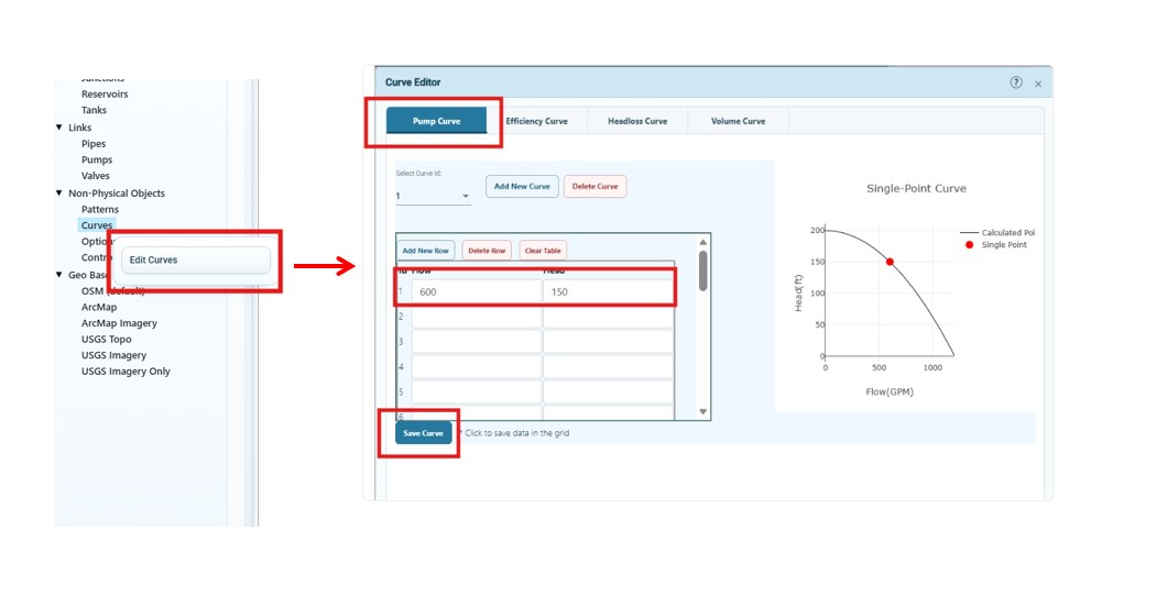
Edit/Define Pump Curve: Non-Physical Objects > Curves > click, right click > Edit Curves
Select the Pump Curve tab from the Curve Editor Window A pump curve ( Curve Id ‘1’ ) is automatically predefined.* Update Flow to 600 GPM and the Head to 150. The software will create a curve through this (pumping rate, head) data point to define the relationship between pumping rate and head in the pump object.**. Click “Save Curve” to finalize the changes. For one point curves the equation used by the software is of the form: ℎ= 𝑏−𝑎𝑄 2 Where h is the Head, Q is the Flow, and b and a are constants determined from the input point(s). *When additional pump curves are needed, click “Add New Curve” button, a new Curve Id (e.g. ‘2’) will appear in the “Curve Id” dropdown box. **Generally speaking, as flow increases, head decreases.
Add Pump Links > Pumps > click, right click > Start Drawing
Again, the cursor turns into a blue circle, indicating ‘Drawing Mode’ is active. Click once on Reservoir 1 to snap the pump’s starting position to it. A blue line will extend from the reservoir as you move the cursor. Double click on Junction 2 to snap the pipe’s ending position to it. *A pump must have a starting and ending node. “Bad” pumps are deleted from the map display. If you get a thin blue line this indicates the link was unsuccessful. When this happens click “Undo” on the map toolbar, or “Stop Drawing” and “Start Drawing” on the Link menu.
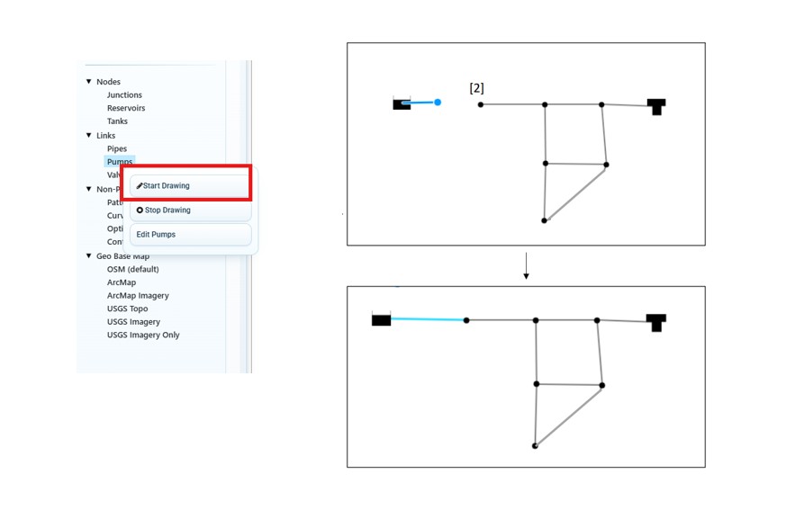
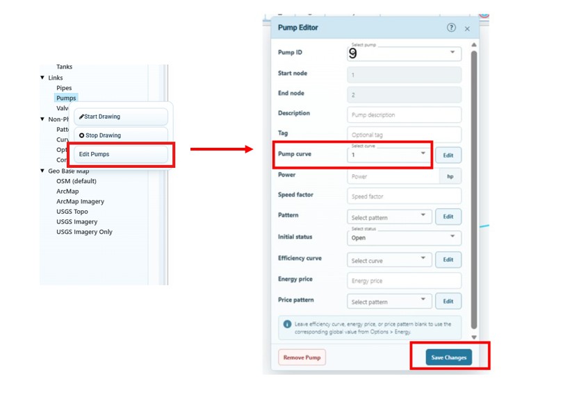
Edit Pump: 1. Links > Pumps > click, right click > Stop Drawing 2. Links > Pumps > click, right click > Edit Pumps
Select the pump using the Pump ID (9 for this example). Assign a ‘Pump Curve’ of 1 (see previous slide). Make sure the ‘Speed’ field is null/empty. Click ‘Save’ to finalize the changes before closing the Pump Data Editor.
5Simulation Options & Demand Patterns
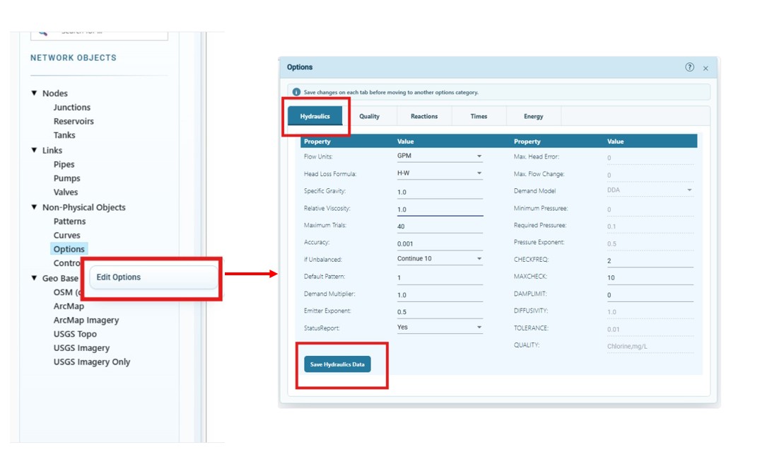
Non-Physical Objects > Options > click, right click > Edit Options Click the “Save” button on each Tab if changes are made to the data in that Tab
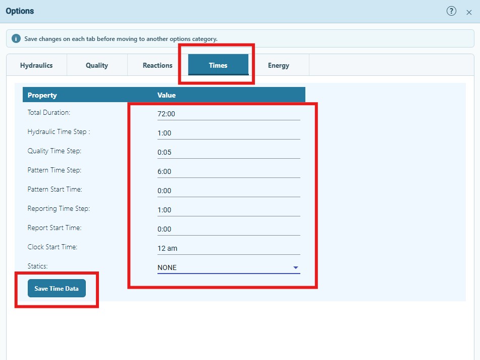
Edit Time Settings: Set simulation time settings and define how demand varies over time.
Navigate to the ‘Times’ tab. Assign a Total Duration of 72 hours (72:00). (This means the analysis will be for a 3-day time period) Assign a Pattern Time Step 6 hours (6:00). (This means demand will be specified in 6-hr increments). Click ‘Save Time Data’ before closing the Options interface.
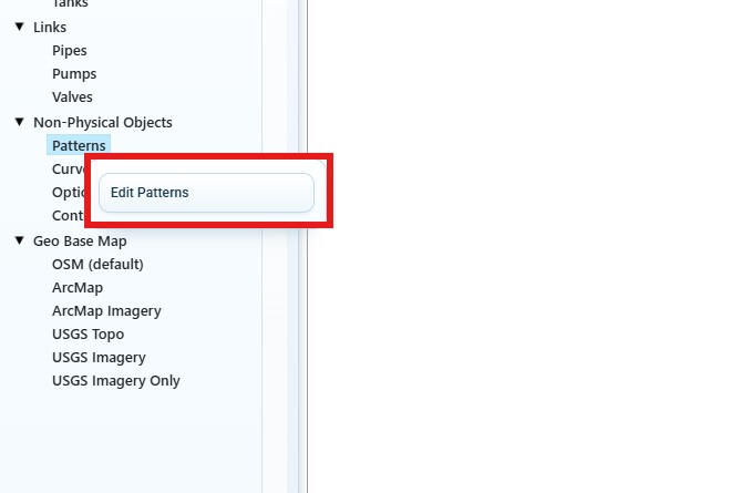
Define Demand Pattern: Non-Physical Objects > Patterns > click, right click > Edit Patterns
Select Pattern 1 from ‘Pattern Id:’. A default demand pattern is automatically provided. *Note that actual demand is product of Base Demand and the Multiplier, where Base Demand is defined in the Junction Data Editor.
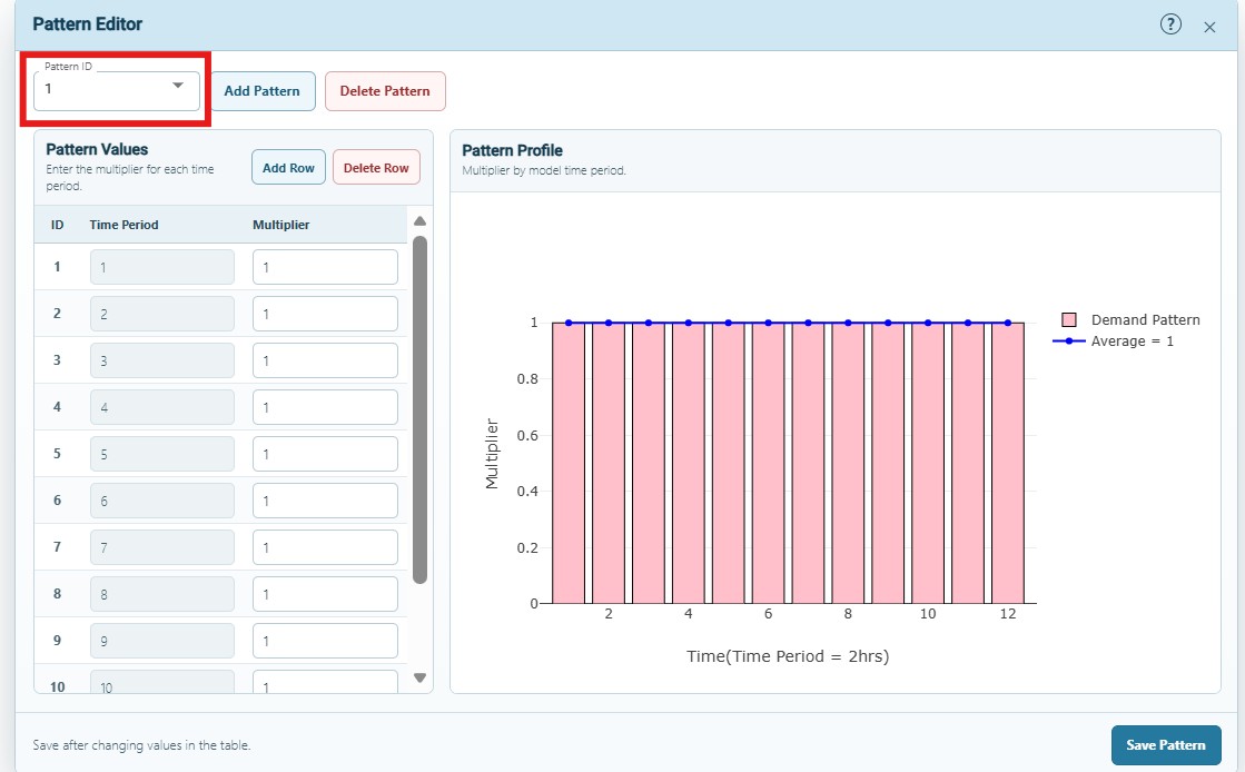
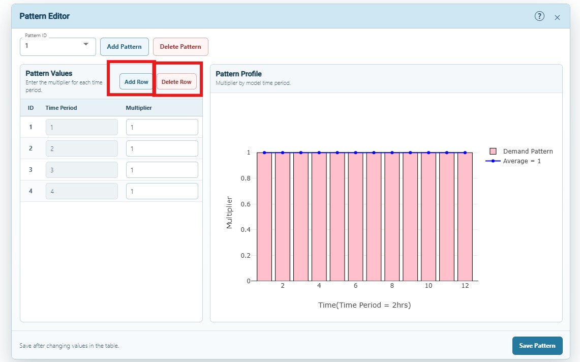
Use the “Delete” button to modify the default pattern (remove all but 4 rows)*. * The “Add New Row” button can be used to add rows if more too many rows are deleted.
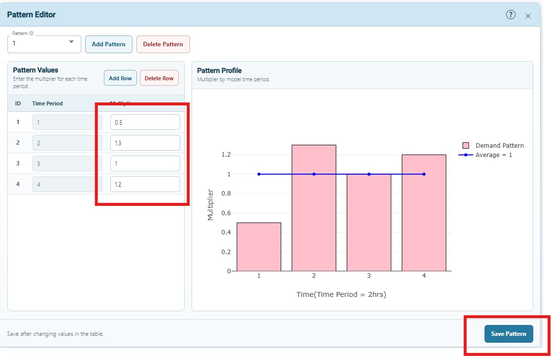
Assign a Multiplier of 0.5 for Time Period 1, 1.3 for Time Period 2, 1.0 for Time Period 3, and 1.2 for Time Period 4. Click ‘Save Pattern’ to save changes.
6Run the Simulation
Execute the hydraulic simulation and check for errors.
Run Model: [Menu Bar] PROJECT > Run Analysis
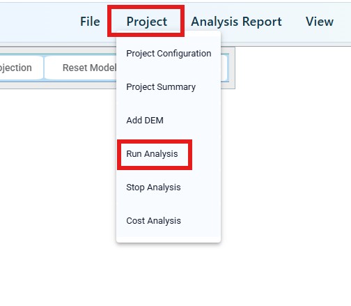
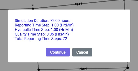
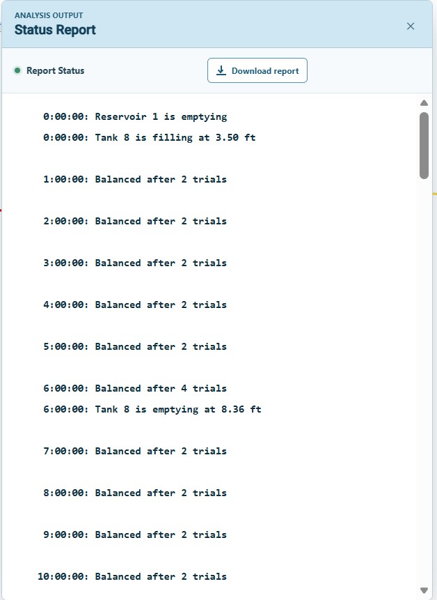
After the model is executed, the Status Window will appear. This window indicates if there were any errors found in the model, and if the model is balanced (water coming in equals water going out), among other information, at different times.
7Visualize Results
Double-click nodes to plot time series, use the Browser Window to color-code the map, view profile plots.
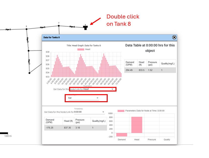
Visualize Results for the Tank: Double-click on the Tank map symbol
This launches the Data for Tanks interface for the tank (Tank ID 8). Select ‘Head’ from the ‘Parameter’ drop-down menu. This creates a time-series of the head (water level) in the tank as a function of time (0 to 72 hours). Select ‘8:00:00’ from the ‘Timestamp’ drop-down menu. This generates a bar chart of the results for four key model parameters (demand, head, pressure, and water quality) at 8 hours of simulation*. *Note that the demand is negative at this time-stamp because the tank is losing water as it provides supply to the pipe system.
Visualize Results Across the Network: Go to Browser Window (automatically generated after Run Analysis)
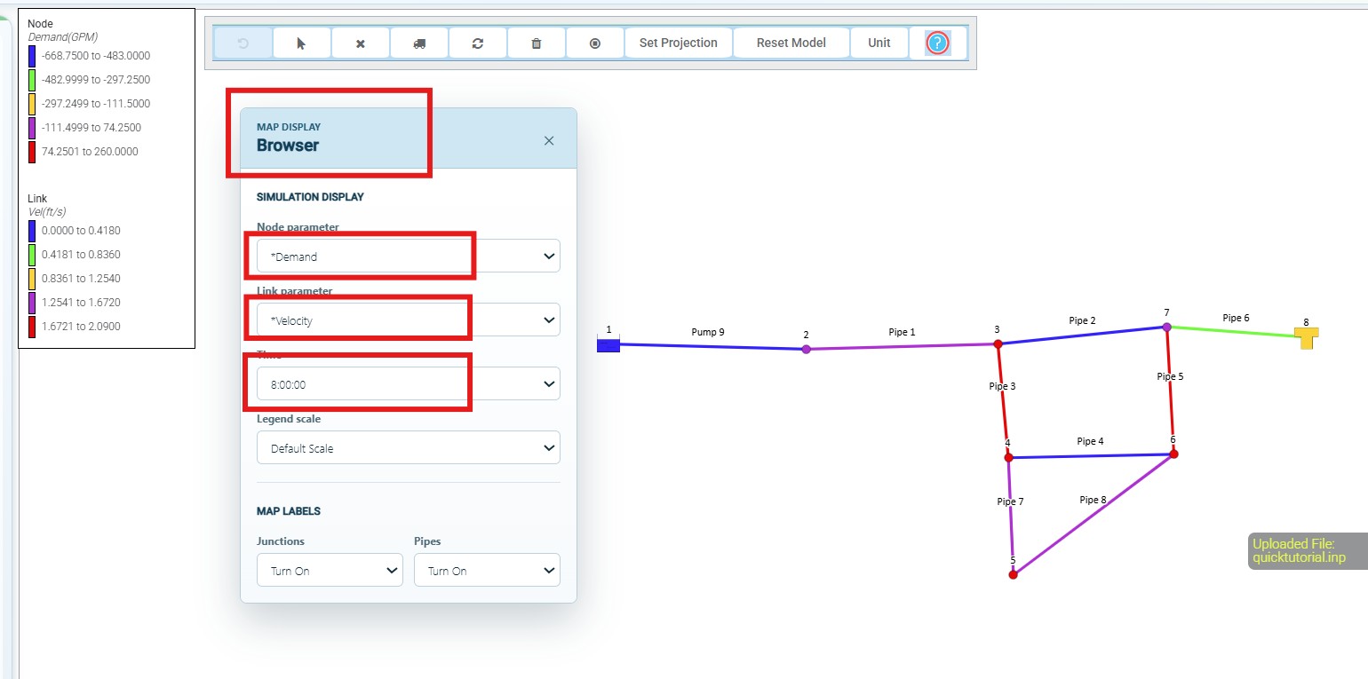
*You may need to close/move the Status Window to see it. Or browse so: View > Map Browser. Select ‘*Demand’ as the Node Parameter. Select ‘*Velocity’ as the Link Parameter. Select ‘8:00:00’ as the Time. The map objects will then be color-coded based on the parameter values at 8 hours of simulation. Note the legend that automatically appears.
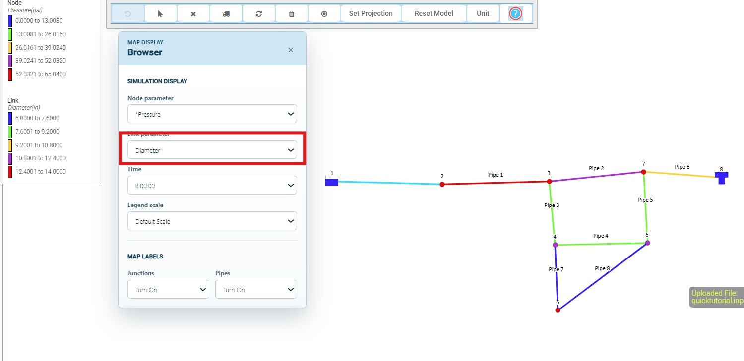
You can also view some of the model inputs, e.g., the diameters of the pipes.
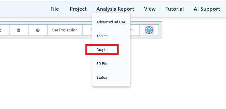
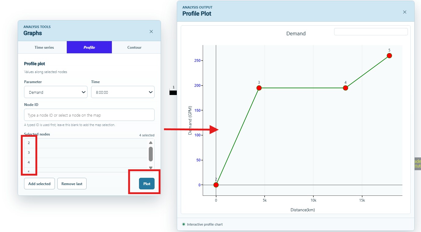
Visualize Results Along a Profile: [Menu Bar] ANALYSIS REPORT > Graphs
This launches the ‘Graphs Window’. Select the ‘Profile’ tab. Double-click on the Junction 2, or enter 2 in the Node input box and then click ‘Add’. This will be the first object along the profile. (Note the ‘2’ add under ‘Selected Features’).
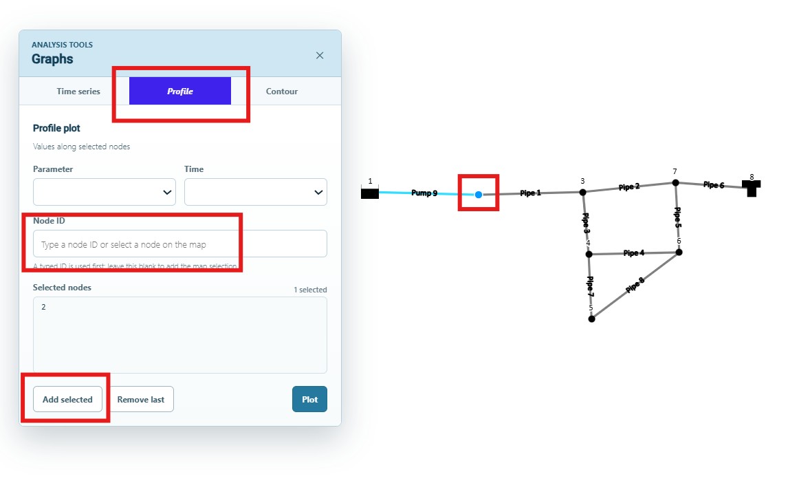
Continue adding Junctions 3, 4 and 5 in the same manner Junction 2 was added. Choose ‘Demand’ from the ‘Select Parameters’ drop-down menu. Choose ‘8:00:00’ from the ‘Select Time’ drop-down menu. Click ‘Plot’. This generates a profile graph of the demand at each Junction (2-5).
83D Visualization
3D pipe network visualization with animated time progression.
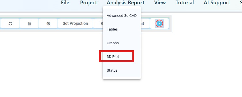
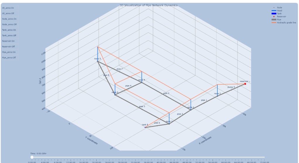
Visualize the Network in 3D Report > 3D Plot
This opens the ‘3D Visualization of Pipe Network Dynamics’ – a 3D rendering of the physical network (pipes and nodes) as well as the simulated parameters (head and hydraulic grade line). *Users can turn on or off any of the 3D plot features using the button palette along the left side of the plot display. ** Use the glider at the bottom of the interface to control the time-stamp for which results are displayed. ***Hover the mouse over any of the pipe features to show parameter values / results.
9Save, Export & Support
Download your model, save the INP file, and contact support for questions.
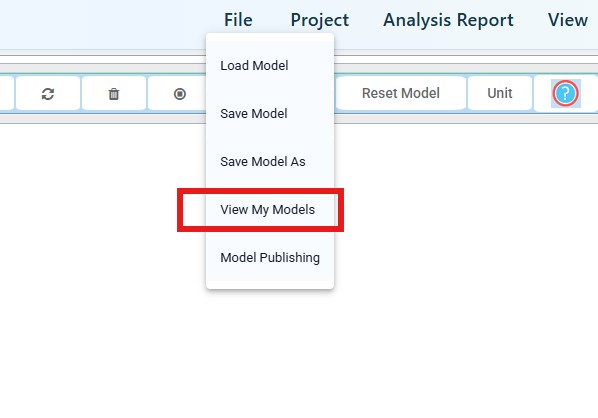
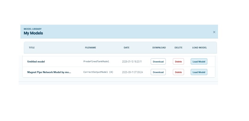
View/Download the Model File: [Menu Bar] FILE > View My Models
This opens a My Models interface. You can select from Saved Models (i.e., those created from File > Save Model …) or Ran Models (previously executed models linked to your user account). Select Ran Models and click Refresh List. In the list that appears Click ‘Download Model’ to download your latest .inp (model input) file to your local machine’s Downloads folder.
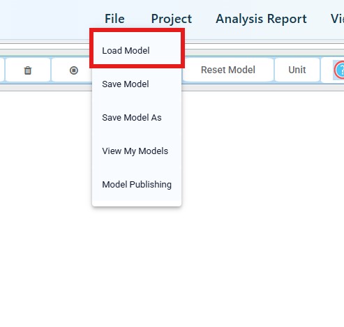
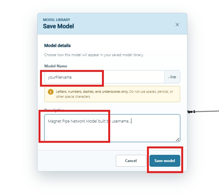
Saving the Model File: [Menu Bar] FILE > Save Model As
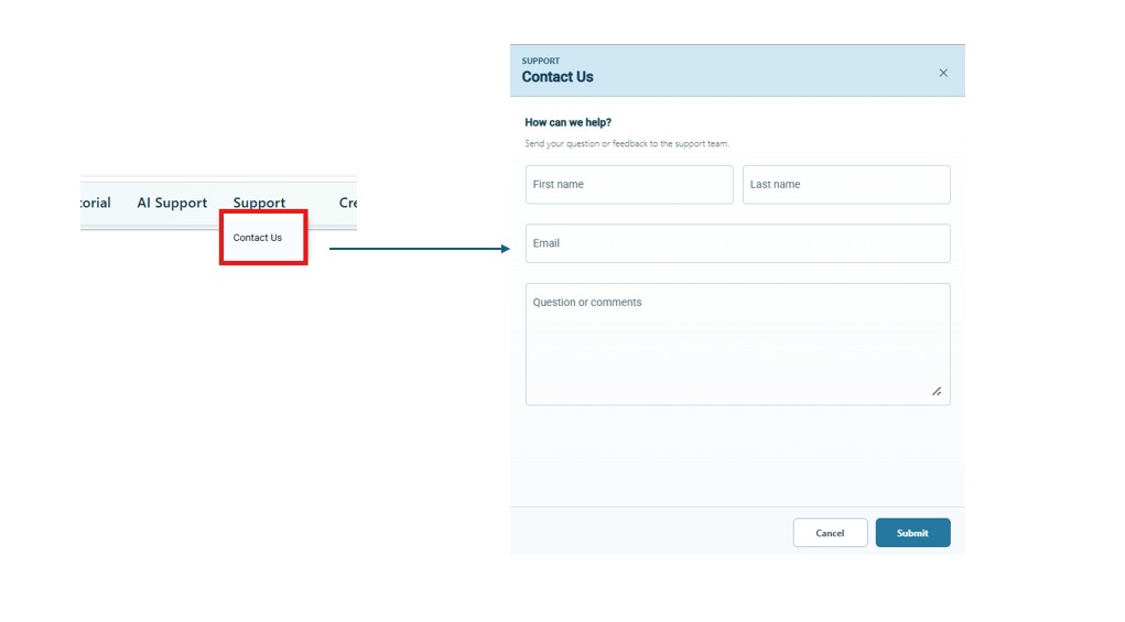
Questions / Comments / Issues?