1Overview — why borehole visualization matters
Groundwater modeling depends on accurate subsurface characterization, and the best evidence for subsurface structure is often water-well driller's logs — hundreds of thousands of logged boreholes across state water-well databases (ODNR in Ohio, EGLE in Michigan, USGS NWIS nationwide). Each log is a vertical sequence of lithologic descriptions ("red clay", "gravel", "sandstone", "weathered bedrock") with depth-to-top, thickness, and sometimes other attributes. DataNET turns these records into 3D colored cylinders in Globe View, standing above (or below) the land surface at each well location.
1.1 The four-class lithology scheme
DataNET classifies every logged material into one of four hydrogeologic classes — a pragmatic scheme that collapses hundreds of lithologic descriptions into aquifer-level categories a groundwater modeler can act on:
| Class | Code | What it means |
|---|---|---|
| AQ | AQ | Aquifer — sand, gravel, coarse permeable sediment or bedrock; primary water-bearing units |
| MAQ | MAQ | Marginal aquifer — silty sand, fine sand, weathered or fractured rock; water-bearing but limited yield |
| PCM | PCM | Partially confining material — sandy clay, mixed fine sediments; restricts but doesn't stop flow |
| CM | CM | Confining material — clay, silt, till, shale; impedes vertical flow |
Each borehole cylinder is rendered as vertically stacked colored segments — one segment per logged lithology interval, colored by its class. A glance reveals the subsurface architecture: thick AQ sequences where the aquifer is well-developed, stacked CM confining layers where aquitards separate flow systems, wedged MAQ/PCM transitions where aquifer connectivity is ambiguous.
2Find the layer and subset your area
For this tutorial we'll use a borehole data layer from the State of Ohio water well database.
2.1 Search for the layer
- Open the Data Layer Library:
- Enter
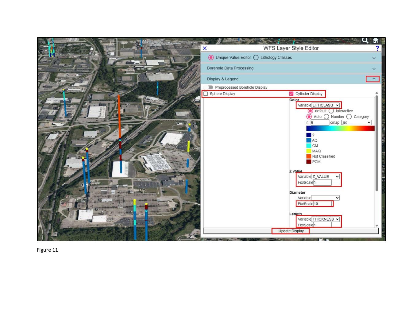
Ohio Lithologyas the keyword, and click Get Layers. - After the search results load, sort layers by Category and expand Groundwater — Borehole Records.
- Find North America Water Well Lithologies (or an Ohio-specific layer). Check the box next to the layer name.
- Borehole locations appear in plan view as red dots (Figure 1).
2.2 Zoom and subset
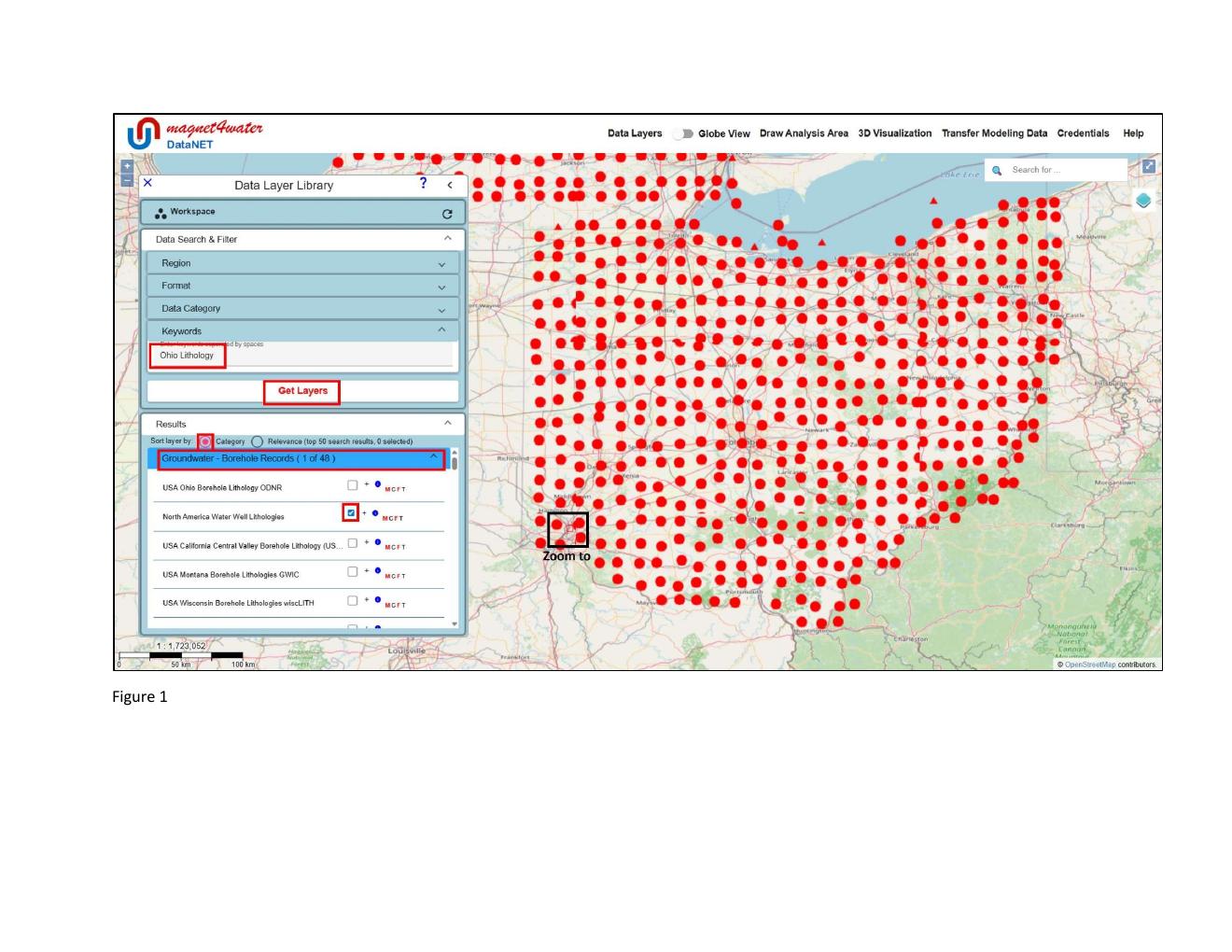
Borehole 3D visualization is computationally intensive, so always subset first. Zoom into the area just north of Cincinnati along Mill Creek. Draw a small rectangular analysis area:
- Click-drag from one corner to the opposite corner.
- Close the draw mode with the same menu entry again.
3Load the boreholes into Globe View
3.1 Switch to Globe View and hide the draped WMS
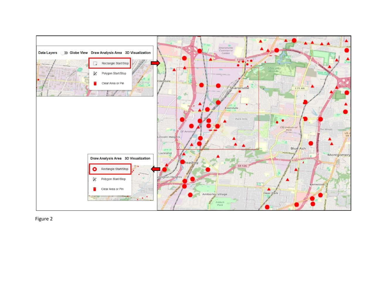
Toggle Globe View on. The Ohio layer initially drapes onto the terrain with its default WMS styling. We don't want that — we want the boreholes standing in 3D, not painted on the ground.
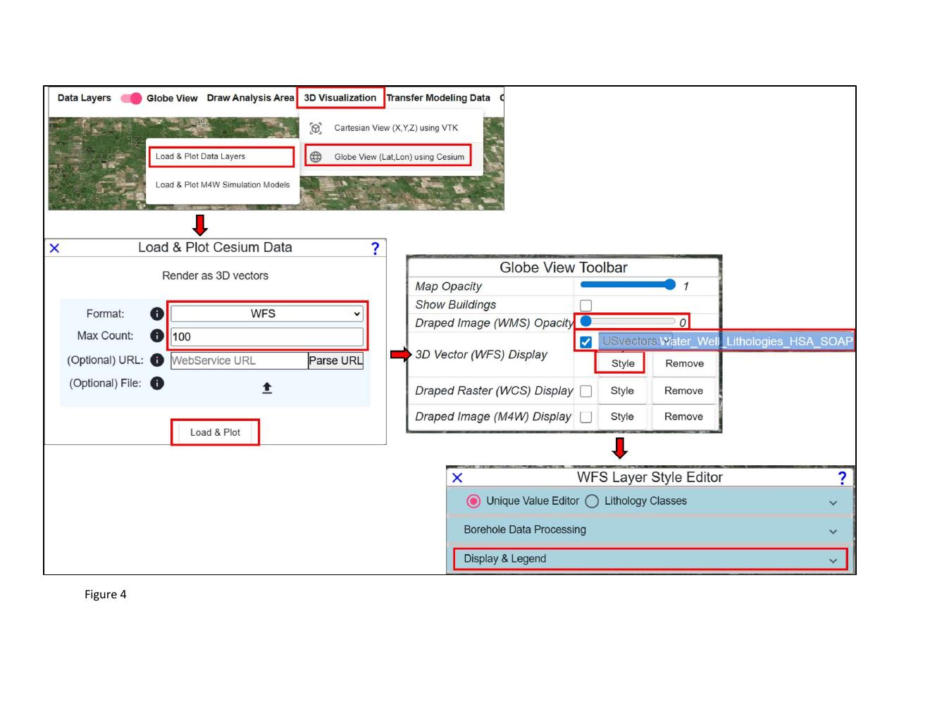
- In the Globe View Toolbar, set Draped Image (WMS) Opacity to zero. The WMS rendering disappears (Figure 3).
3.2 Load and plot the 3D vectors
With the WFS layer still checked in the Data Layer Library:
- In the Load & Plot Cesium Data dialog, select Format: WFS.
- Optionally set Max Count to under 100 to avoid browser memory overload on large subsets.
- Click Load & Plot.
After loading, the Globe View Toolbar shows a new entry in the 3D Vector (WFS) Display area. Click Style to open the WFS Layer Style Editor (Figure 4).
4Preprocessed Borehole Display (standardized datasets)
Here's where DataNET's hydrogeology workflow pays off.
4.1 The standardized format
Many regional borehole datasets in DataNET are already in a standardized schema where each feature has four canonical fields:
WELLID— unique well identifierELEV— material top elevationTHICKNESS— material thicknessLITHMAT— substrate material type, pre-classified to one of AQ MAQ PCM CM
For these datasets the work is already done — DataNET knows how to render them in 3D.
4.2 Toggle the Preprocessed Borehole Display
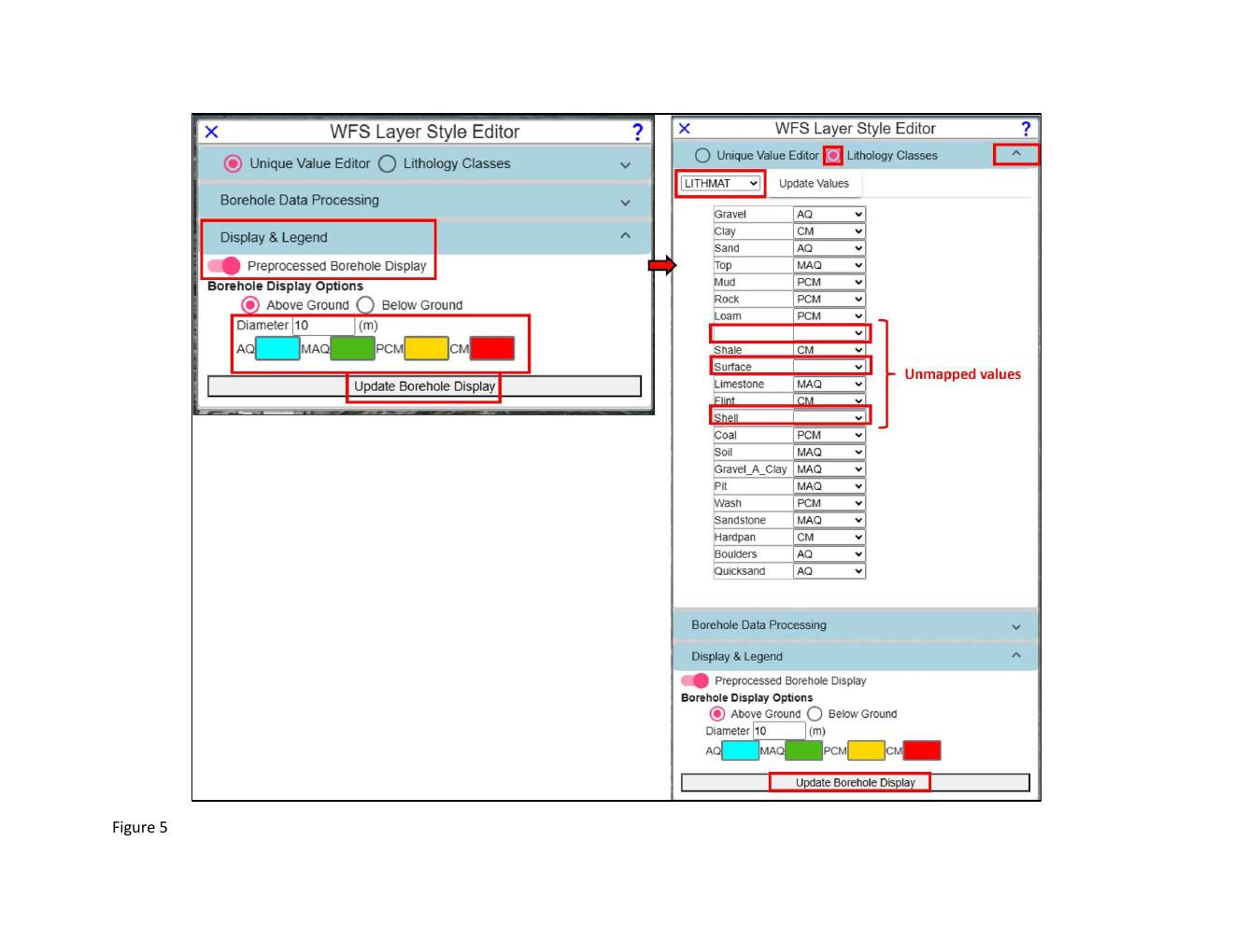
- In the WFS Layer Style Editor, expand Display & Legend.
- Click the Preprocessed Borehole Display toggle (Figures 4 and 5).
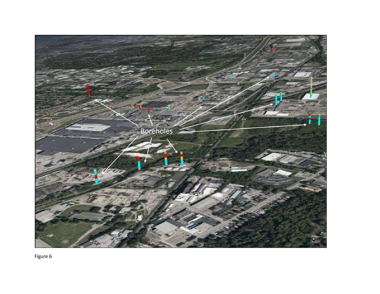
Each borehole now renders as a vertical stack of cylinders, one per logged lithology interval, colored by material class. Zoom in to see the subsurface architecture emerge — where Aquifer layers stack thickly, where confining material pinches out, where marginal-aquifer transitions fingered through the section.
4.3 Customize if needed
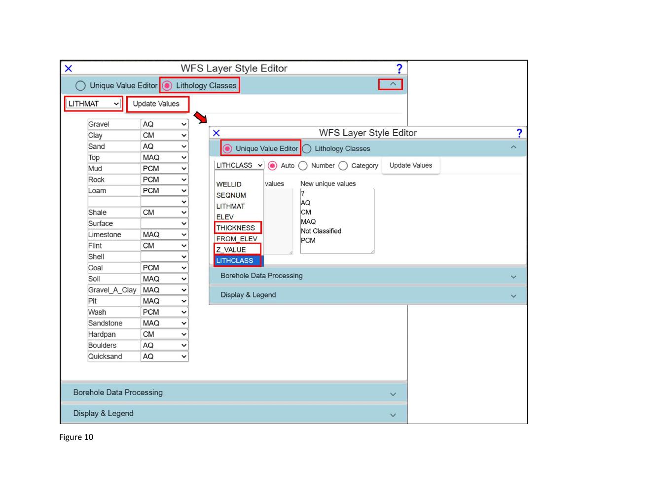
You can optionally edit the default borehole diameters or the material-class colors, then click Update Borehole Display to refresh (Figures 5 and 6). You can also view and edit the underlying lithology-to-class mapping by selecting Lithology Classes, expanding the section, and selecting the LITHMAT attribute — a full table of original lithologic descriptions mapped to the four-class scheme. Some datasets may have unmapped entries; you can reassign them or override the default mapping here.
4.4 Click a borehole for details
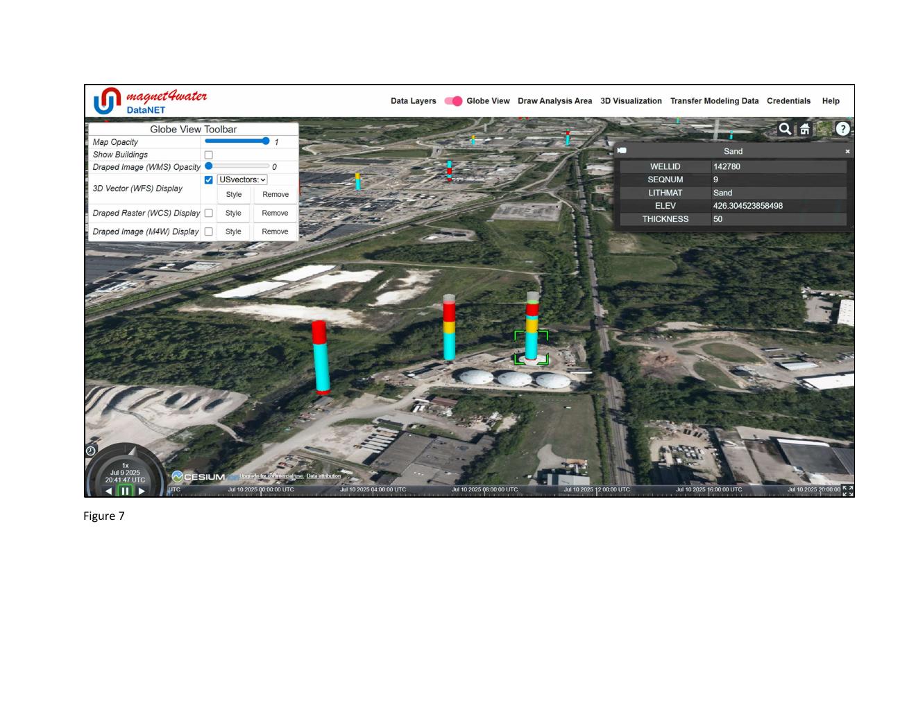
Clicking on any interval of any borehole reveals the full feature attributes — well ID, top elevation, thickness, original lithologic description, and any additional fields from the source dataset (Figure 7). This keeps the raw geology available even when viewing the four-class simplified display.
5Above-ground vs. below-ground display
By default, boreholes stand above the land surface like colored pins — great for a quick overview, but not physically accurate. For subsurface modeling context, switch to below-ground mode.
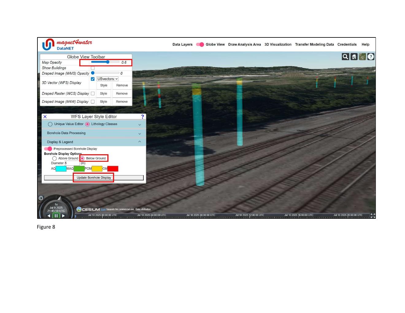
- In the WFS Layer Style Editor, select the Below Ground option.
- Boreholes now extend downward from the land surface into their actual depth.
- To see them underground, lower the Globe View Map Opacity below 1.0 — the terrain becomes semi-transparent, revealing the boreholes in their true subsurface position (Figure 8).
6Custom datasets — Borehole Data Processing
Not every borehole dataset arrives in the standardized WELLID / ELEV / THICKNESS / LITHMAT format. You might have: a state dataset with depth from / depth to instead of elevation + thickness; a layer with a free-text material column and no class assignment; a private log export with non-standard column names. DataNET handles all of these via the Borehole Data Processing tool and the Lithology Classes mapping table.
6.1 Get to know the data
- Click the ⓘ info button next to the layer (in the Data Layer Library or Workspace) — check the metadata for attribute names and units.
- Click on the spherical WFS features in Globe View — inspect the attributes of a sample feature.
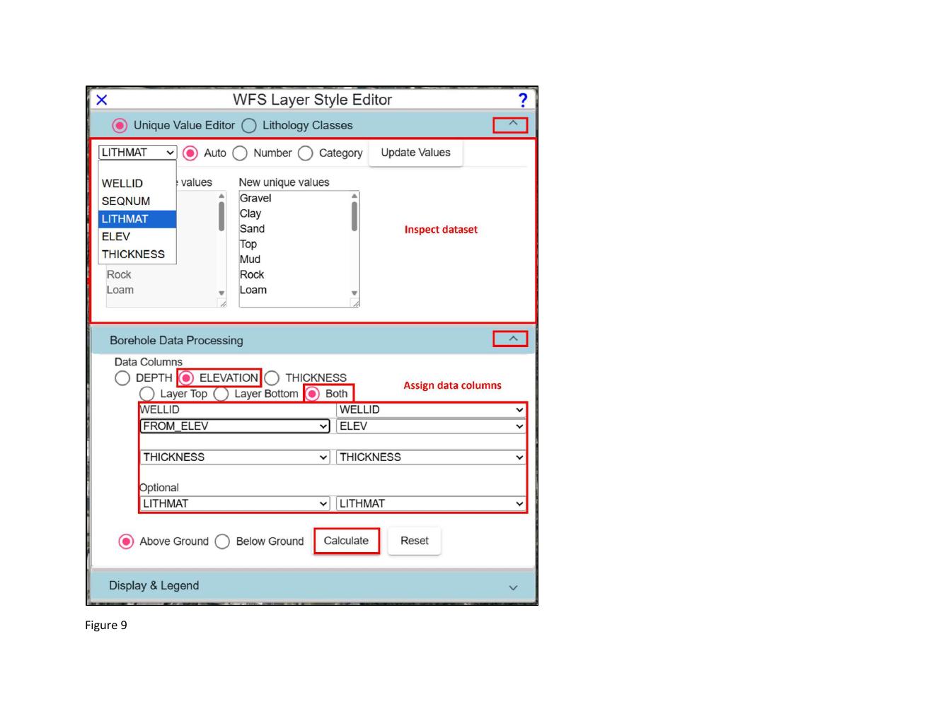
- In the WFS Layer Style Editor, expand the Unique Value Editor section — see what each attribute actually contains (Figure 9).
6.2 Process: define the elevation reference
- Expand the Borehole Data Processing section.
- Choose a reference scheme based on your data's structure:
- Depth — if the dataset has depth-from / depth-to for each interval
- Elevation — if the dataset has absolute top/bottom elevations
- Thickness-only — if only thickness is given
- Many datasets specify depth from and depth to. For the North America Water Well Lithologies layer we have both top elevation (
ELEV) and thickness (THICKNESS), so we choose Elevation for the reference and Both since we have the two relevant fields. - Assign your dataset's columns to the calculation variables:
WELLID,FROM_ELEV,THICKNESS, and optionallyLITHMAT. Click Calculate (Figure 10).
6.3 Build a LITHCLASS field
- Expand the Lithology Classes section.
- Choose the source field (e.g.,
LITHMATor the dataset's own material-description column). - Make any needed changes to the mapping table — assign each unique lithology name or description to one of AQ MAQ PCM CM.
- Click Update Values.
6.4 Check the required fields are present
After calculating values and mapping lithology classes, verify everything DataNET needs is now available. In the Unique Value Editor, confirm the required computed fields show up with reasonable values:
Z_VALUE— the top elevation of each intervalTHICKNESS— interval thicknessLITHCLASS— the four-class hydrogeologic category you just mapped
6.5 Update the display with your mapped fields
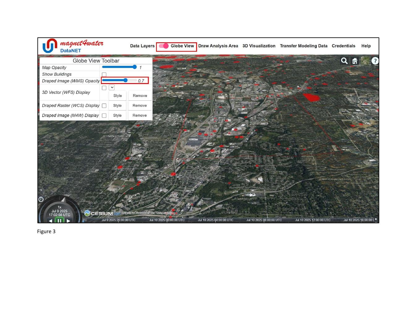
- Expand Display & Legend.
- Uncheck Sphere Display, check Cylinder Display.
- Select
LITHCLASSas the Color Variable. - Select
Z_VALUEas the Z value Variable,THICKNESSas the Length Variable. - Optionally tune Fix/Scale values (the Z value and Length must have the same scale to avoid overlapping cylinders).
- Click Update Display (Figure 11).