1Overview & find the time-varying layer
DataNET supports the OGC standard for time-varying WMS — known as WMS-T — which lets you step through or animate raster map data across time. Examples include radar reflectivity, satellite imagery sequences, climate model output, and time-stamped satellite-derived products.
Layers that can be animated are marked with an animation icon next to the layer name in the Data Layer Library or Workspace. If you don't see the icon, the layer is static (no time dimension available).
Finding a WMS-T layer
For this tutorial, we use the World NEXRAD BASE REFLECT layer — NOAA's Next-Generation Radar base reflectivity product, time-stamped and continuously updated.
- Open the Data Layer Library:
- Keyword search for
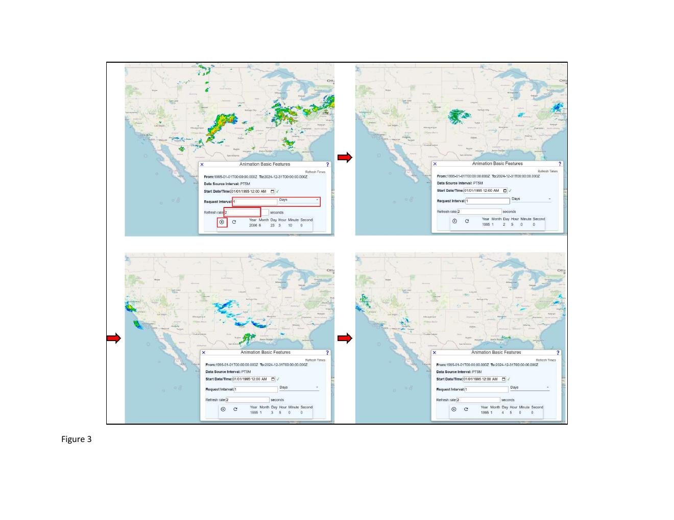
NEXRAD, or navigate to the National Aeronautics & Space Admin Animation category. - Find the World NEXRAD BASE REFLECT WMS layer.
- First, check the box next to the layer name to see the static (current-moment) plan-view rendering — this confirms the layer loads correctly before you animate (Figure 1).
2The Animation Basic Features interface
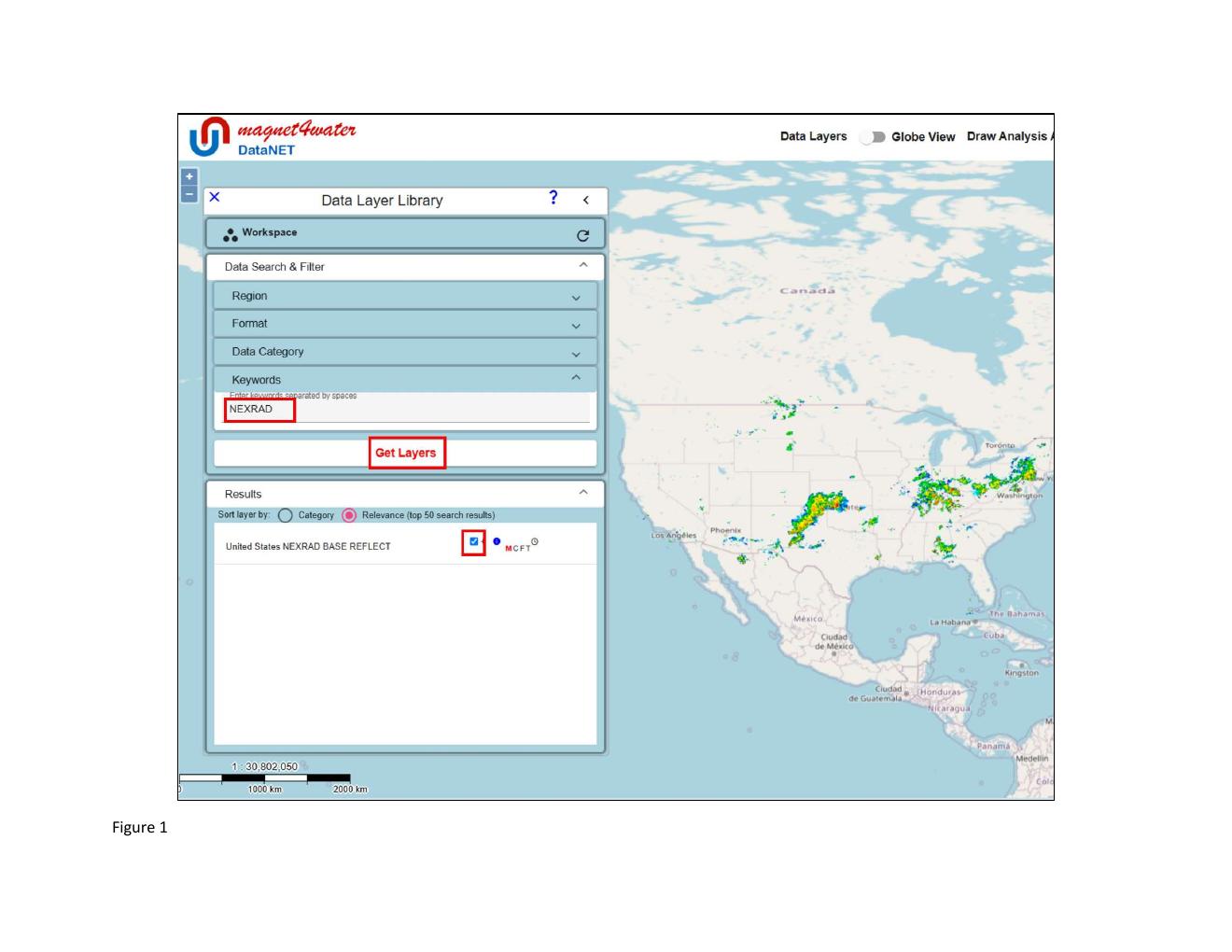
With the layer visible, click the animation icon next to the layer name to open the Animation Basic Features interface (Figure 2). It has four controls:
| Control | What it does |
|---|---|
| Start Date/Time | When to begin the animation. Must be within the data source's available time range. |
| Request Interval | The time-step to increment the animation between frames. This must be a multiple of the source data interval — asking for 1-minute frames from a 15-minute-interval source wastes requests and gets you duplicate frames. |
| Refresh Rate | How many seconds each frame displays before advancing. Sets the playback speed. |
| Pause / Resume | Stop and restart the animation playback. |
The Animation interface also shows the From: and To: date/time range of available data — your Start Date/Time and the resulting animation must fall within this range.
A future release will also allow customizing the end date/time of the animation so you can focus on a specific subset of the overall data duration.
3Configure and play the animation
The NEXRAD layer updates at short intervals (often every 5–15 minutes of real time). At that cadence, flipping through sequential frames shows very little change — weather doesn't move that fast at continental scale. To see clear evolution of storm systems, step through at a coarser interval.
3.1 Set a meaningful interval
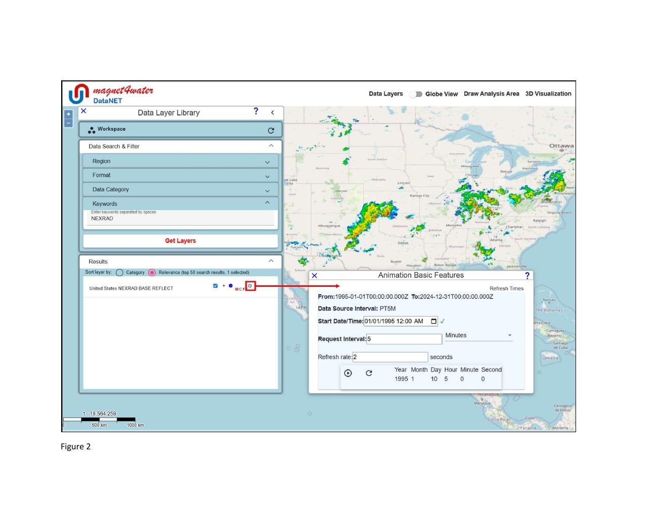
- Change Request Interval to
1 day. Now each frame jumps 24 hours into the future. - Change Refresh Rate to
2 seconds. Each day holds on screen for 2 seconds before advancing (Figure 3).
3.2 Play back and observe
Restart the animation (click the play icon). The map redraws every 2 seconds with the NEXRAD reflectivity pattern for the next day in the sequence. Watch storm systems sweep west-to-east across North America, and how the overall spatial pattern of precipitation concentration shifts over days.