1Overview
DataNET offers two complementary ways to visualize map data (WMS images with no underlying vector or raster values):
- Plan view — the traditional 2D map display, best for scanning a wide region and for overlays with clean spatial alignment
- Globe View — a full 3D environment powered by Cesium, where WMS layers drape onto a global digital terrain model. Best for seeing how data relates to topography, and for any follow-on 3D visualization workflows.
This tutorial walks through both, plus how to combine multiple WMS layers into a coherent thematic overlay.
2Toggle background maps
In both plan view and Globe View, several background basemaps are available. Click the Background Map icon (control D from Tutorial 10) to switch between options:
- OSM (default) — OpenStreetMap
- ArcMap — ArcGIS basemap
- ArcMap Imagery — ArcGIS satellite imagery
- USGS Topo — USGS land-surface topography (great for hydrology context)
- USGS Imagery — USGS satellite imagery with labels
- USGS Imagery Only — USGS satellite imagery without labels (cleaner for publication)
- Water Color — Stadia Maps stylistic basemap
- Blank Map — plain white — lets your thematic WMS layers stand alone
Globe View has its own independent basemap options (see §4 below).
3Display a layer in plan view
The first step is always to find a layer of interest. Layer search is covered in detail in Tutorial 1.
For this example, we'll visualize a global data layer: World Mean Precipitation…
- Open the Data Layer Library:
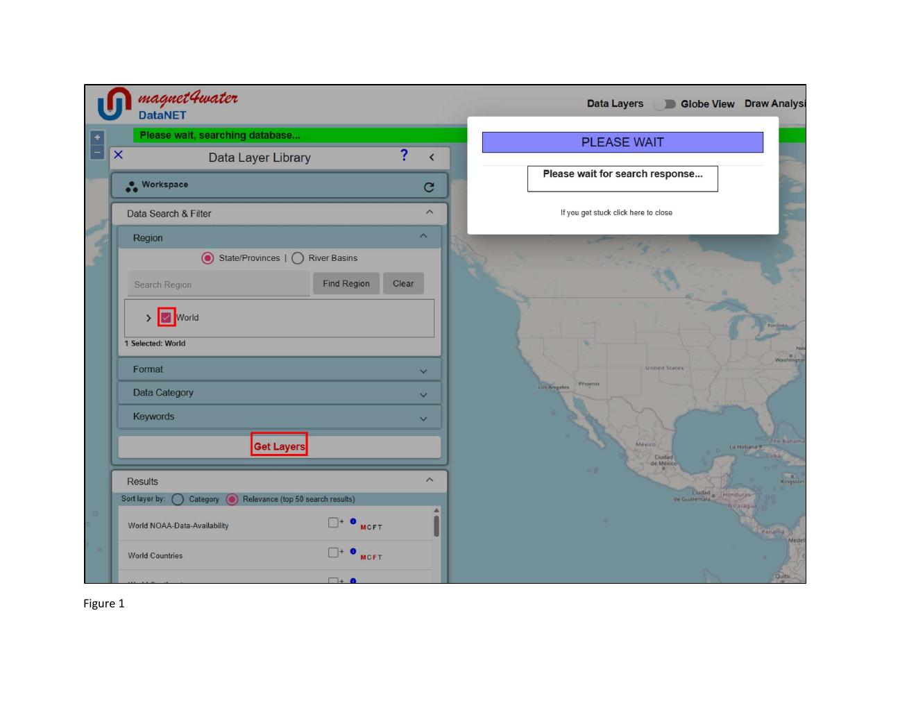
- Check the box next to World in the Region filter and click Get Layers.
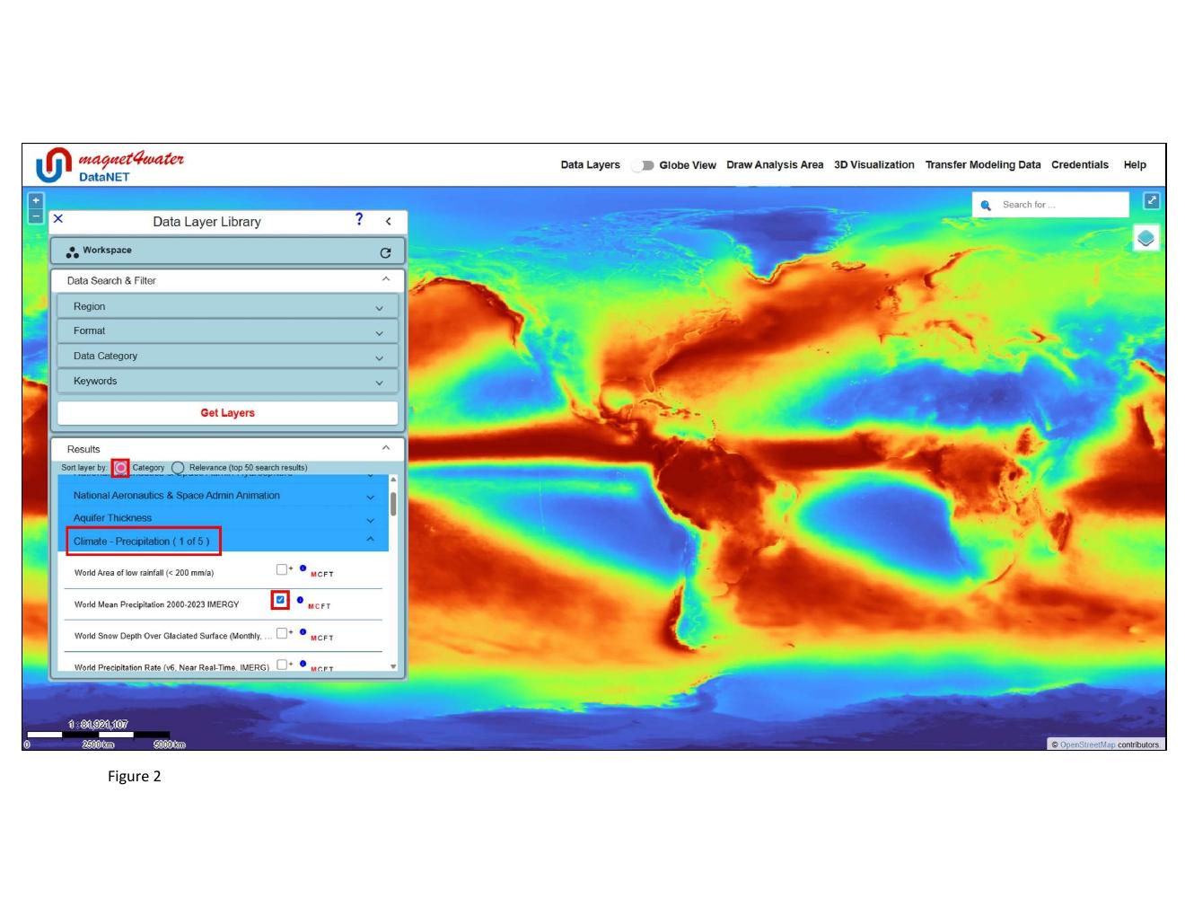
- Sort the retrieved layers by Category.
- Expand Climate — Precipitation and find World Mean Precipitation… (see Figure 1).
- Check the box next to the layer name. The layer loads into the plan-view map display after a few moments (very high-resolution datasets can take longer — be patient).
4View the layer in Globe View
With the layer still checked, use the Globe View toggle (control F) in the DataNET Title Bar to instantly convert the mapping environment into 3D mode. The global precipitation layer is automatically draped onto the Cesium digital terrain model.
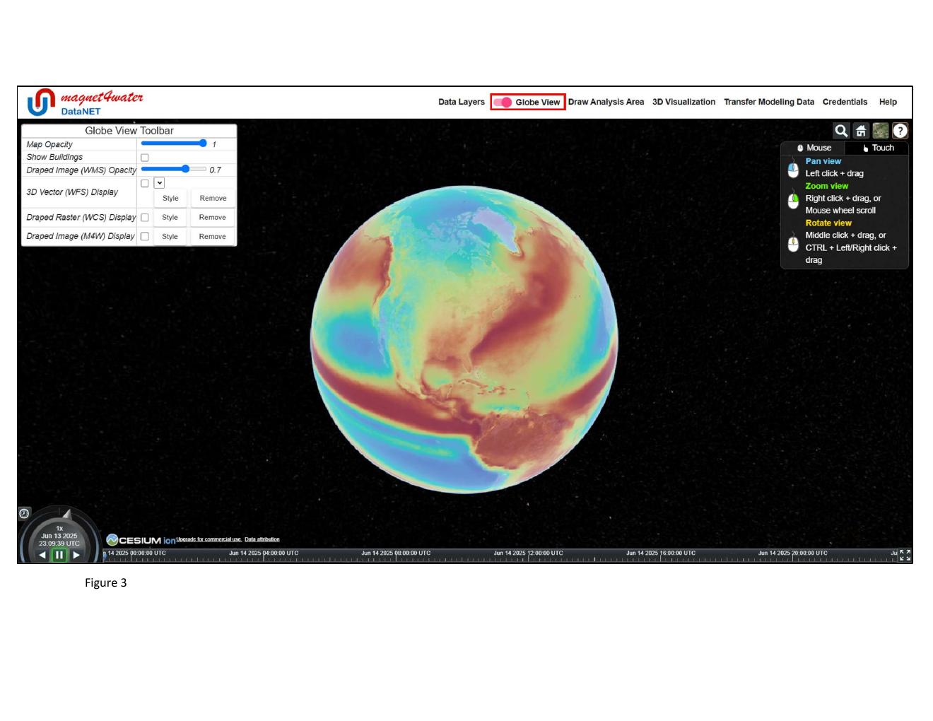
Globe View has its own set of display options accessed from the Globe View Toolbar — layer transparency, basemap selection, optional real-world buildings (for urban views), and more. These are covered in Tutorial 7 (Globe View WFS Styling) and Tutorial 13 (Borehole Lithologies).
5Build a multi-layer overlay
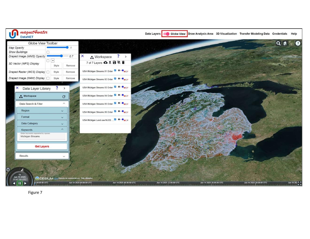
Next we demonstrate displaying multiple WMS layers as an integrated overlay — in this example, Michigan land use underneath Michigan stream layers.
5.1 Toggle off Globe View and clear the Library
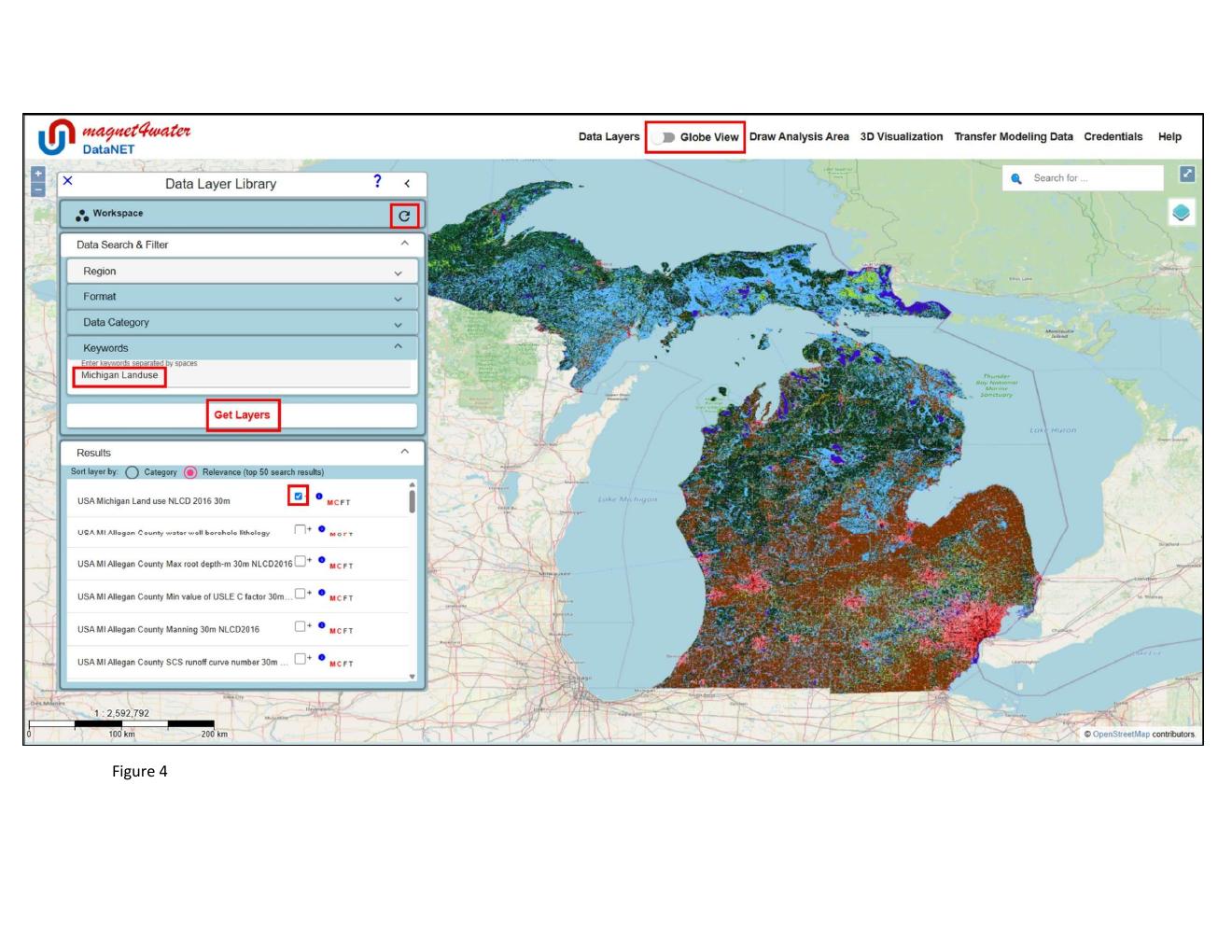
- Toggle Globe View off (click control F again).
- Open the Data Layer Library and clear it (using the reset icon).
5.2 Search and add the land-use layer
- Keyword search for
Michigan Landuse(see Tutorial 1 for search details). - Find and check the USA Michigan Land use… layer (Figure 4).
5.3 Start a Workspace
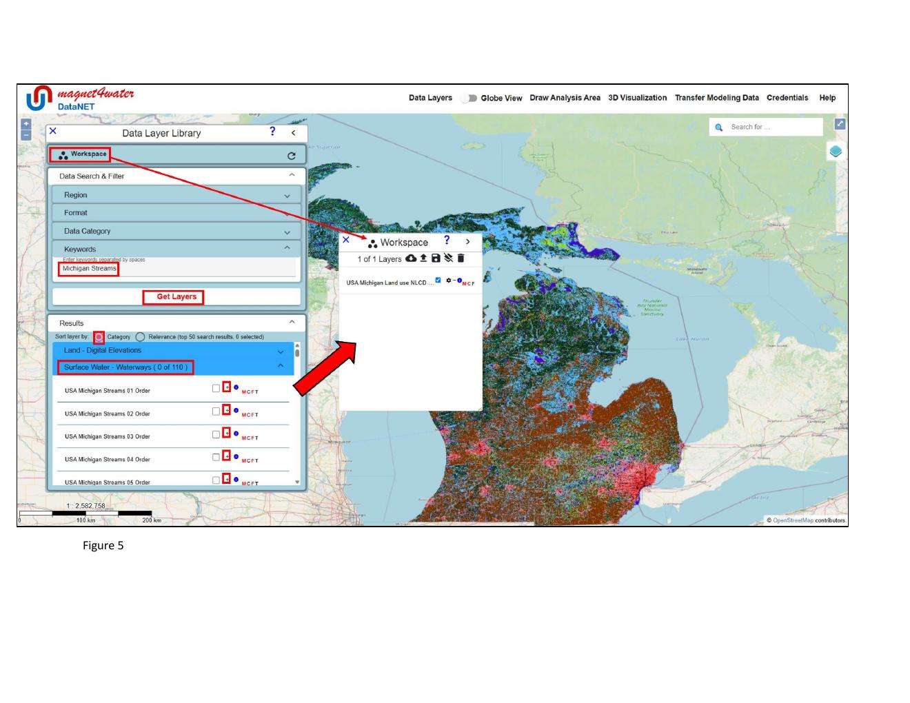
- Click Workspace in the Data Layer Library interface to start a new Workspace.
- Click the + icon next to the Michigan land-use layer to add it to the Workspace.
5.4 Add the stream layers on top
- Now keyword search for
Michigan Streamsand find them in the Surface Water — Waterways category. - Add each USA Michigan Streams layer to the Workspace (different number suffixes are different stream orders / sizes — see Figure 5).
- When prompted, place the stream layers on top of the Workspace so they render over land use.
5.5 Reorder if needed and render
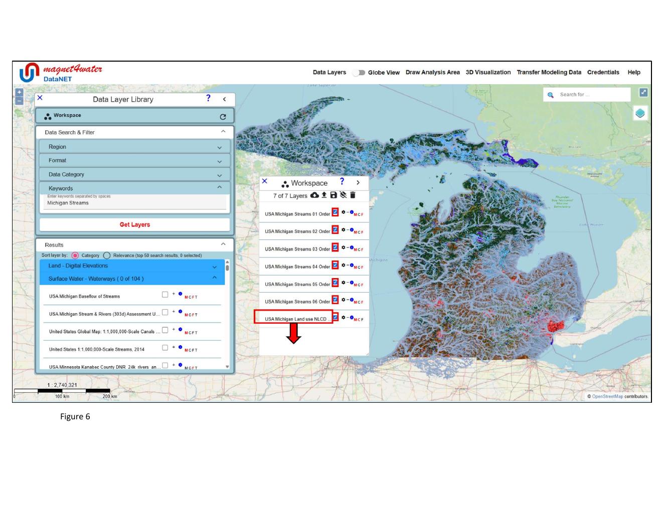
Workspace layers can be reordered by dragging up and down. If needed, drag the land-use layer to the bottom so it renders behind the streams. You can also grab the handle in the bottom right corner to resize the Workspace panel.
Check all the layers in the Workspace. The overlay builds in the plan-view map display (Figure 6).
5.6 View the overlay in Globe View
Toggle Globe View back on. The complete multi-layer overlay is automatically draped onto the Digital Terrain Model — you get a 3D view of the thematic composite.