The quick read — 90 seconds
- The domain is a 2D polygon on the web map. Everything you do afterward — aquifer attributes, zones, lines, wells — is defined inside it. You cannot resize or reshape the domain after you add features, so choose deliberately.
- Four drawing methods: DomainRect (rectangle, fastest), DomainPoly (arbitrary polygon), DM from a txt File (vertices from a text file, for reproducibility), DM from a shapefile (GIS-standard import, for precise study-area boundaries).
- Size the domain generously. Leave 2-3 km of buffer between your site of interest and the domain boundary. For a specific site, draw a regional domain (10-30 km), then use a submodel for the detailed local work. Too small is worse than too large: undersizing means the no-flow boundaries distort the flow field at your site.
- The default boundary condition is no-flow on all four sides and the bottom. This assumes your domain is drawn large enough that lateral boundaries are far from the area of interest, and that the bedrock below is effectively impervious compared to the surficial aquifer.
- Accept the suggested projection (almost always UTM) unless you have a specific legacy-system reason not to. Groundwater equations need meters, not latitude/longitude.
- If your first domain turns out too small or the wrong shape, don't try to redraw it. Start a fresh model, use what you learned to draw the new domain better, and rebuild from there. For localized refinement that wasn't planned, use a submodel — that's always allowed.
4.1 What the Domain Is
Before you draw anything, it helps to understand exactly what role the domain plays in your model — and why its boundaries matter so much.
4.1.1 The domain defines the extent of computation
The domain is the 2D polygon outlining the region where IGW-NET will solve the groundwater flow equation. Inside the domain, every grid cell has a computed head, a computed concentration (if transport is active), and contributes to the water balance. Outside the domain, there is nothing — the platform does not track what happens beyond your boundary.
This is different from a "map" in a GIS. A GIS map shows features in a geographic region; the region has no physical meaning beyond display. An IGW-NET domain is a physical region — the boundary is a hydrogeologic boundary, and what that boundary represents (no-flow, prescribed head, specified flux) directly shapes the solution.
4.1.2 The domain fixes everything else
Once the domain exists, every other element of your model is defined inside it or relative to it:
- Aquifer attributes (Ch. 5) — top, bottom, K, recharge, storage — apply across the domain's area.
- Zones (Ch. 6) are polygons inside the domain that override domain attributes locally.
- Lines (rivers, drains, boundary conditions) are traced inside the domain.
- Wells are placed at points inside the domain.
- Particles are released from locations inside the domain.
- Grid cells tile the domain's bounding rectangle at your chosen NX resolution.
Because every feature is defined relative to the domain, you cannot resize or reshape the domain after adding features — the coordinate system of the features is anchored to the domain you drew. If you try, IGW-NET will not let you, and if it somehow did, the features would no longer make sense.
If your first model reveals that the domain should have been larger, or a different shape, the practical path is: save your work, start a new model, draw the new domain better, and rebuild the features. This is annoying but usually quick — features accumulate fast once you know the workflow. The exception is localized refinement — if you just need more detail in one spot, draw a submodel inside the existing domain. That's always allowed (see §4.6 and Ch. 13).
4.2 The Four Drawing Methods
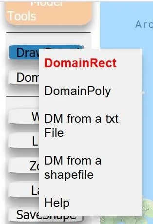
IGW-NET offers four ways to define a domain, accessed through the DomainRect dropdown in the Conceptual Model Tools panel. Each suits a different situation.
| Method | Speed | Precision | Best for |
|---|---|---|---|
| DomainRect | Fastest (click-drag) | Rectangular only | First models, regional scoping, any case where a bounding rectangle captures your area of interest. 80% of IGW-NET models start here. |
| DomainPoly | A few minutes of clicking | Arbitrary shape | Irregular study areas — watersheds, catchments with natural boundaries, jurisdictions with non-rectangular limits, aquifer systems with complex shapes. |
| DM from a txt File | Instant after file ready | Arbitrary, to numerical precision | Reproducibility across collaborators or sessions — everyone uses the same vertex list. Also useful for scripted workflows that generate domain files programmatically. |
| DM from a shapefile | Instant after upload | Matches your GIS | When your study area is already defined in a GIS (watershed, wellhead protection area, property boundary, permit area). Most professional work moves to this method eventually. |
4.2.1 DomainRect — the default choice
For almost any new model, start here. DomainRect is simple: click the button, then click-drag on the web map to draw a rectangle around your area of interest. A confirmation dialog shows the extent; click OK to accept.
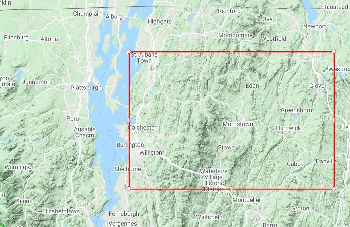
Rectangles have practical advantages beyond speed. They align with the grid cells the solver uses, so there are no partial boundary cells to worry about. They capture a generous area with minimal drawing effort. And they force you to think about the bounding box of your study area, which is usually the right scope for a first model.
4.2.2 DomainPoly — for irregular shapes
When the bounding-box approach wastes too much area on features you don't care about, use DomainPoly. Click to start, then click each vertex along the boundary you want. Double-click (or click the starting vertex) to close the polygon.
Watersheds are the classic case. A watershed has a natural boundary — the topographic divide — that rarely aligns with a rectangle. Drawing a polygon that follows the divide produces a much more relevant model area.
Other good cases: coastal modeling where you want to exclude ocean area, aquifer systems bounded by distinct geologic units, permit boundaries, and jurisdictional areas (a county, a tribal land boundary).
4.2.3 DM from a txt File — for reproducibility
For collaborative or reproducible work, DM from a txt File lets you define the domain as a list of longitude-latitude vertex pairs in a simple text file. One vertex per line, comma-separated, in the order the polygon is traversed. Upload the file and the domain is drawn exactly.
This is the right choice when:
- Multiple team members need to build models on the same domain — everyone uses the same text file.
- You're running a scripted workflow that generates domain definitions programmatically.
- You want to document the exact domain in a publication or technical report — the text file can be included as a supplement.
4.2.4 DM from a shapefile — the GIS bridge
For GIS-based workflows, DM from a shapefile accepts a standard polygon shapefile (.shp plus the companion .dbf, .shx, .prj files, typically zipped). The platform reads the polygon and uses it as your domain — preserving the exact boundary defined in your GIS.
Typical sources for domain shapefiles:
- Wellhead protection area boundaries from a regulatory agency
- Property boundaries for site-specific investigations
- Watershed boundaries delineated in a GIS using DEM analysis
- Permit boundaries for mining, waste disposal, or extraction projects
- Pre-defined study areas from a larger research program
Two things to watch for when importing: (1) Projection — shapefiles carry their own projection in the .prj file, and IGW-NET will honor it; if the shapefile is in a projection other than lat/lon, IGW-NET will still handle it correctly, but make sure the .prj file is present. (2) Multi-polygon shapefiles — if your shapefile contains multiple polygons (e.g., multiple islands), you may need to dissolve them into a single polygon or pick the one you want before importing.
4.3 Choosing the Size
The single most common mistake new users make is drawing the domain too small. Understanding why — and how to think about sizing — saves many rebuilds.
4.3.1 The rule of buffering
Your domain should be larger than your area of interest — usually much larger. The reason: the default boundary condition is no-flow (§4.4), which means water cannot cross the boundary. If your site of interest is close to a no-flow boundary, the simulated flow field near your site will be distorted by that artificial constraint. Heads pile up behind the boundary; flow deflects away from it. Your site sees a flow field that doesn't reflect reality.
The fix is buffering: draw the domain so that between your site of interest and the nearest boundary, there is enough distance for boundary effects to dissipate. A practical rule:
For most regional groundwater systems, leave at least 2-3 km of buffer between your site of interest and any domain boundary. For highly permeable aquifers (gravels, karst) where flow can be fast and far-reaching, increase this to 5+ km. For site-scale work focused on a specific property, err even more generously — and plan to use a submodel for the detailed analysis.
4.3.2 Recommended sizes by problem type
| Problem type | Recommended domain size | Why |
|---|---|---|
| Teaching / first model | 5-10 km on a side | Big enough to capture regional flow patterns, small enough to simulate quickly. Perfect for learning. |
| Regional water-resources study | 20-50 km on a side | Captures watershed-scale drainage patterns, major rivers, regional divides. |
| Wellhead protection for a single well | 10-20 km regional domain + submodel | Regional domain establishes context; submodel provides detailed capture-zone analysis. |
| Contaminant plume tracking | 5-15 km regional + submodel | Site-scale resolution for the plume; regional context for upgradient and downgradient features. |
| Property-scale investigation | 5-10 km regional + submodel | Always use a regional parent. A property-scale domain alone will have artificial boundary effects everywhere. |
| Watershed-scale ecological study | Watershed polygon (DomainPoly) | Use the natural watershed boundary; topographic divide acts as a natural no-flow boundary, which is physically correct. |
4.3.3 The trade-off with simulation speed
Larger domains take longer to simulate. At the default grid resolution (NX=40 cells on the long axis), a 10 km × 10 km domain simulates in seconds; a 100 km × 100 km domain might take a minute. Doubling the domain dimension roughly doubles simulation time — not a severe penalty. The real trade-off isn't speed; it's resolution. A fixed NX spread over a larger domain produces coarser cells, so regional features are less crisply resolved. This is exactly why submodels exist: regional context at coarse resolution, local detail at fine resolution, each optimal for its purpose.
4.4 The Default No-Flow Boundary
The platform's default boundary condition deserves careful understanding — it shapes every simulation's result in ways that aren't immediately obvious.
4.4.1 What "no-flow" actually means
By default, IGW-NET treats all four lateral boundaries of your domain — plus the aquifer bottom — as no-flow: water cannot cross them. This is a specified-flux boundary condition with flux set to zero.
For the bottom, this assumption is usually fine. The default aquifer bottom is set to represent the top of bedrock (or the equivalent confining unit), which typically has hydraulic conductivity orders of magnitude lower than the aquifer above it. Treating it as no-flow introduces negligible error — you'd need to specifically care about deep groundwater exchange to justify refining this.
For lateral boundaries, the no-flow assumption is only appropriate when the domain is large enough that boundaries are far from your area of interest. This is why buffering matters so much (§4.3). If you draw a small domain with your site near the edge, the no-flow boundary creates artifacts that look like real hydrogeology but aren't.
4.4.2 When no-flow boundaries are correct
In some cases, no-flow boundaries are physically correct — not approximations you're willing to tolerate, but genuine reflections of reality:
- Watershed boundaries. Topographic divides are natural no-flow boundaries for the near-surface aquifer, because groundwater flow follows topography in most humid settings. Drawing a domain that matches a watershed makes the no-flow assumption physically defensible at the perimeter.
- Impermeable geologic boundaries. When your domain boundary follows a known impervious fault, a bedrock ridge exposed at surface, or a low-permeability formation contact, no-flow accurately represents the physics.
- Symmetry boundaries. When the flow system has a symmetry axis — a divide centered between two parallel streams, for example — you can place the boundary on the axis and use no-flow to represent that no water crosses an axis of symmetry.
4.4.3 Changing boundary conditions when needed
If the default no-flow boundary isn't what you need, you can override it in three ways:
- Add an explicit polyline along the boundary with a prescribed-head or prescribed-flux condition (Ch. 6 §6.2). This overrides the default for that segment of boundary.
- Use a submodel — draw a smaller domain inside a parent domain, check Boundary Condition from Parent Model, and the submodel's boundaries inherit from the parent's head solution. This is the most robust way to handle boundary conditions for a local model (§4.6 and Ch. 13).
- Draw the domain differently — make it bigger, or reshape it so the boundary lies along features where no-flow is accurate.
Most IGW-NET models use default no-flow boundaries with adequate buffering, and most of those that need something different use submodels. Explicit boundary polylines are reserved for specialized cases.
4.5 Projection — Almost Always UTM
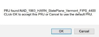
After you confirm the domain, IGW-NET asks you to choose a projection. This sounds technical; in practice it's almost always a single click.
4.5.1 Why the platform asks
Groundwater flow equations — Darcy's law, the continuity equation — are written in terms of distance and gradient. Distance in latitude-longitude isn't meaningful: one degree of longitude is 111 km at the equator but only 55 km at 60° latitude. To compute heads, gradients, and fluxes, the platform needs a coordinate system where distances are in meters.
A projection converts latitude-longitude coordinates into a flat Cartesian system. Different projections distort different things — areas, shapes, distances, or angles — and no projection can preserve all of them at once. For groundwater modeling, you want minimum distance distortion, because that's what the solver uses.
4.5.2 Why UTM is almost always right
Universal Transverse Mercator (UTM) divides the world into 60 zones, each 6° of longitude wide, and each zone has its own Mercator-style projection optimized for that zone. Within a zone, distance distortion is minimal (under 0.04% at the worst). IGW-NET's suggestion algorithm looks at your domain's location and picks the right UTM zone automatically.
For almost every domain, this is the right choice. Click OK and move on.
There are a few specific cases where you might want a non-UTM projection: (1) your domain spans multiple UTM zones — rare at typical modeling scales; (2) you're matching a legacy project that used State Plane, Albers Equal Area, or another system; (3) you're publishing results alongside an agency that requires a specific projection. Otherwise, UTM is correct.
4.6 Planning for Submodels
Even before you've drawn your first domain, it's worth knowing how submodels work — because they shape how you should think about sizing the parent domain.
4.6.1 The submodel workflow
A submodel is a smaller domain drawn inside an existing parent domain. Its boundary conditions inherit from the parent's head solution, and its grid can be much finer than the parent's, so you get local resolution without paying computational cost over the whole regional area.
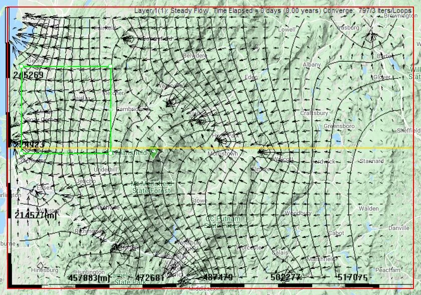
Drawing a submodel takes about one minute:
- Open Zone drawing tools (Draw Zone → ZoneRect)
- Click-drag a rectangle inside the parent domain
- Open the Zone Attributes menu for the new zone
- Check Submodel Domain → Active
- In the parent's Simulation Settings, check Boundary Condition from Parent Model
- Run the submodel — it uses the parent's solution at its boundaries
Chapter 13 covers submodels in depth. The point for now: submodels exist, they are instantaneous to create, and they solve the "I need finer resolution locally" problem without requiring you to resize your domain.
4.6.2 What this means for domain sizing
Because submodels are easy, your parent domain doesn't need to be optimized for local detail. You can (and should) draw it generously to ensure good regional context, knowing that any detailed local analysis will happen in a submodel.
For any site-specific work, plan a regional parent domain sized generously around your site (10-30 km, with 2-3 km buffer), plus a local submodel covering the detailed area of interest. The parent gives you context and proper boundary conditions; the submodel gives you resolution. This two-tier approach is so common and so effective that most production IGW-NET models use it. Planning for it from the start means your parent domain doesn't need to compromise between "big enough for context" and "small enough for detail" — those competing goals are satisfied separately.
To go deeper
- Chapter 5 — Aquifer Attributes — next chapter. Once the domain is drawn, aquifer attributes are what make it a runnable model.
- Chapter 13 — Nested Modeling (Submodels) — the complete submodel workflow.
- Quick Tutorial 2: Nested Modeling — hands-on walkthrough of the parent-submodel workflow.
- Platform Concept: Submodel Boundary Precedence — the important gotcha about how the inherited BC flag resets.
- Case Study: Mancelona TCE — real-world example of the regional-plus-submodel approach.