The quick read — 90 seconds
- IGW-NET always shows a working solution. The moment you define a domain, you have a complete, runnable base model — flow, transport, particles, visualization — all wired up with robust defaults. You're never "setting up" from scratch; you're refining something that already works.
- Defaults prioritize numerical robustness over raw accuracy. The bottom of your aquifer defaults to minimum DEM minus a constant, not the bedrock raster — this keeps cells wet and the solver convergent so you always see a solution to learn from. You refine toward accuracy.
- Every attribute has a customization ladder: typical default → your constant → Data Center raster → your uploaded raster → DataNET service → scattered points with interpolation → T-PROGS 3D geology. You ascend the ladder where visualization shows it matters.
- More variability ≠ more accuracy. Keep it simple. A constant K supported by your data is usually more predictive than a highly variable K field that the data cannot justify. Refine only when data, sensitivity analysis, or the incremental modeling process tells you to. Overly complex models are not better models — they are often just overfit.
- Modeling is incremental by design. Start coarse, 2D, one layer. See what the model tells you. Draw a submodel box (one click: use parent model as BC) and get instant local refinement. Add sublayers and conceptual layers. Trying to build a "correct" model in one shot is the biggest pitfall — when something goes wrong, you won't know where it went wrong.
- Zones override domain. Inside a zone polygon, the zone's attribute values take precedence. Where a zone is silent, the domain fills in. Zones unlock refinement options — scattered-point interpolation, T-PROGS — that the domain alone doesn't offer.
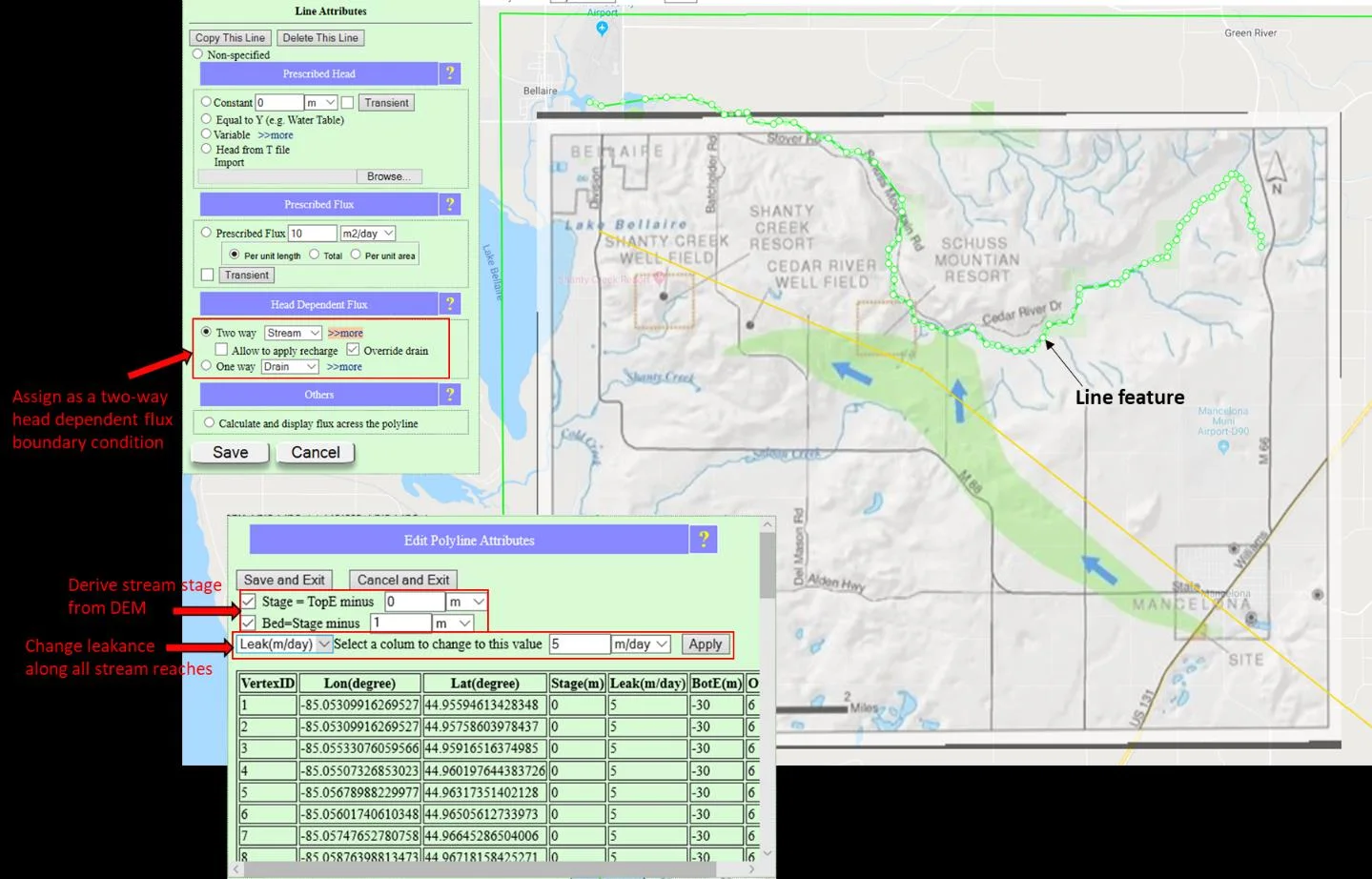
- Leakance units follow geometry, not convention. River (line):
leakance = (Ksed/thicknesssed) × width, unitsm/day. Lake (polygon):leakance = Ksed/thicknesssed, units1/day. Same physics, different integration. - DEM-as-surface-drainage is the default, for a reason. Over a regional area with non-trivial recharge, whatever comes down has to go up — surface water naturally functions as a drain for the groundwater system. DEM-as-drain captures 90%+ of this effect automatically. Refine to explicit rivers and lakes when you need two-way exchange (arid regions, losing streams, large coupled lakes). Larger features become two-way head-dependent; smaller ones stay as one-way drain. None of the defaults are locked in — change any conceptual assumption and the platform immediately visualizes the result.
5.1 The Base Model: What You Get For Free
The most important idea in this chapter — and arguably the most important idea in the entire platform — is that you do not assemble a groundwater model in IGW-NET. You refine one. From the moment you draw a domain, a complete, runnable simulation exists.
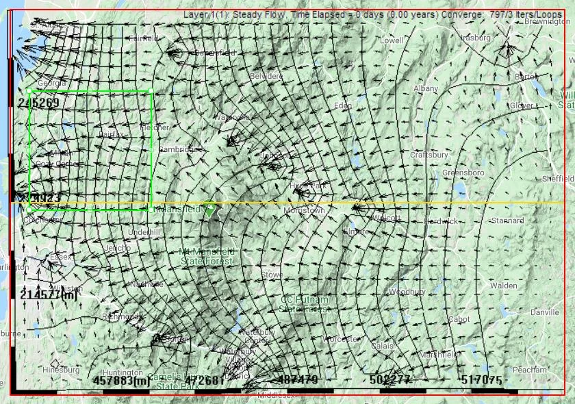
Click SIMULATE and the base model runs. Head contours appear. Velocity vectors appear. Cross-sections can be drawn and color themselves with vertical conductivity. A water balance tracks where water enters and leaves. Add a concentration source anywhere, and transport activates automatically — you see the plume migrate. Drop a zone of particles on the flow field, and a particle animation starts — you see where water actually goes.
5.1.1 What the base model represents
By default, the base model simulates natural groundwater conditions in the near-surface, unconfined, water-table aquifer — the shallow aquifer system that drives water supply and sustains groundwater-dependent ecosystems (wetlands, springs, baseflow to streams, and riparian vegetation). This default focus is deliberate: near-surface aquifers are where most real-world groundwater questions live, and they are where the platform's design choices pay off most clearly.
Specifically, the base model:
- Represents the aquifer top as the spatially-variable land surface from the Data Center DEM — 90 m globally via ASTER Global DEM, 30 m or 10 m in the USA via USGS NED.
- Predicts where the water table intersects the land surface as part of the solution process itself — not as a post-processing step. This is what makes the base model's head distributions qualitatively accurate even with typical defaults: the topography-driven discharge pattern into wetlands, springs, and seeps is baked into how the solver works, not added on afterward.
- Treats the aquifer bottom and lateral boundaries as no-flow, assuming the underlying bedrock is effectively impervious compared to the surficial aquifer, and that the domain is drawn large enough that lateral boundaries don't influence the area of interest. (If you need lateral boundary conditions from a larger regional model, that's what submodels are for — see §5.10.)
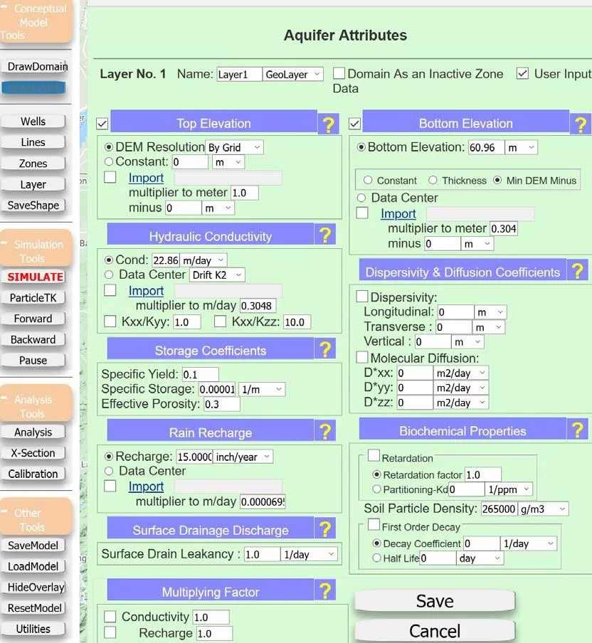
- Uses a single effective recharge and single effective hydraulic conductivity across the domain — typical values chosen for numerical robustness — which you then refine along the customization ladder.
If you have used published models from the MAGNET4WATER Observatory, this base-model description will feel familiar — every published model starts with these same default assumptions about the near-surface, unconfined water-table aquifer. What's different now: the platform's model parser reads your specific model and generates a description tailored to what you have actually built. Where the legacy description said "a single effective value for recharge is used," the parser-driven description can tell you exactly which Data Center raster you chose and what multiplier is in effect. The users' manual and the parser-driven descriptions share the same core vocabulary — so concepts you learn here map directly onto the reports your deployed models generate.
5.1.2 Why the base model exists
Most groundwater modeling tools treat setup and simulation as separate phases. You enter values, configure boundaries, pick a solver, and then run — hoping you didn't miss anything. When something is missed, you face a blank screen or a cryptic error, and debugging can take days.
IGW-NET inverts this. The platform assumes you will forget things, misconfigure things, and simulate before you are "ready." It handles those realities by giving you a complete, runnable model from click one. The model is always prepared to simulate. Your role is to refine it toward accuracy, guided by what the visualization shows you at each step.
Seeing a solution — even an approximate one — is worth more than debugging a crash. When the solver converges, visualization tells you what's right and what needs refinement. When it doesn't converge, you learn nothing. IGW-NET is designed so the solver always has a chance of converging — by giving every parameter a numerically robust default. Refinement becomes a guided conversation with the visualization, not a blind configuration exercise.
5.1.3 End-to-end from click one
The base model is not just flow. It is the complete pipeline:
- Flow: Darcy's law solved over your grid with default K, recharge, and boundaries. Heads, gradients, velocities.
- Transport: Dormant until you add a source. Add one — concentrations activate automatically, and you get an animated plume.
- Particles: Dormant until you add a particle zone or a particle-releasing well. Add one — you get animated pathlines following the flow field.
- Analysis: Charts for water balance, cross-sections, head hydrographs at any point, concentration breakthrough at monitoring wells — all automatically populated as the solver runs.
- Visualization: Plan view, cross-sections, 3D views — updated in real time as the simulation advances.
All of this comes from defaults. You did not configure any of it. You drew a domain; you clicked simulate; you see the system. That's the base model.
Plumes, particles, and animated flow reveal the system in ways that static head contours cannot. Watching a particle navigate around a pumping well, or a plume deflect along a stream, teaches you what the flow field means far faster than any chart. The base model gives you that insight as quickly as possible — because insight, not calibration, is the primary product of groundwater modeling.
5.2 The Customization Ladder
Every aquifer attribute — top, bottom, K, porosity, storage, recharge — follows the same refinement pattern. You start at a low rung (a typical default) and climb toward accuracy only when visualization shows the low rung isn't enough.
Not every attribute has all seven rungs. Hydraulic conductivity has all of them. Surface drainage discharge in practice has only rungs 0 and 1. The table at §5.9 shows which rungs apply to which attributes.
Most successful models live at rung 2 or 3 (Data Center or uploaded raster) for the critical parameters and at rung 0 (default) for everything else. Climbing the ladder has real cost — uploading data, capturing borehole logs, calibrating interpolation — but the deeper cost is conceptual: more variability does not mean more accuracy, and often means less.
A highly variable K field that the available data cannot support is not a better model than a well-chosen constant. It is an overfit model, and overfit models are unreliable predictors. The principle is sometimes called KISS: keep it simple and stupid. Use the simplest conceptual model that allows you to meet your objectives. Refine only when (a) you have new data that justifies the added complexity, (b) IGW-NET's real-time sensitivity analysis shows the refinement matters, or (c) the incremental modeling process has revealed a specific need. Climb the ladder slowly and for good reasons. Complexity has to earn its place.
5.3 Top Elevation
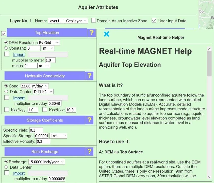
The simplest of the seven attributes. The top of your aquifer is almost always ground surface, and ground surface is almost always well-represented by the Data Center DEM.
| Rung | Setting | When to use |
|---|---|---|
| 0 (default) | DEM Resolution: Auto (By Grid) | Anywhere. This is the right answer for ~95% of real sites. |
| 0 (variant) | DEM: 10m / 30m / 90m explicitly | When you want finer or coarser DEM than the auto match to grid. |
| 1 | Constant value | Synthetic or teaching models where a flat aquifer helps communication. |
| 3 | Import your own raster | You have a higher-resolution DEM than the Data Center provides (e.g., LiDAR). |
If your model cell size is 200 m, there is no benefit to a 1-m DEM — the extra detail is smoothed away by grid averaging. "Auto (By Grid)" picks the right resolution automatically. Changing it is worth the thought only if your cells are very small (< 30 m) or very large (regional).
5.4 Bottom Elevation
This is where the "robust defaults" philosophy shows most clearly. The default is not the most physically realistic choice — it's the one that guarantees the solver converges. Understanding why will help you refine intelligently.
5.4.1 The default: minimum-DEM-minus-constant
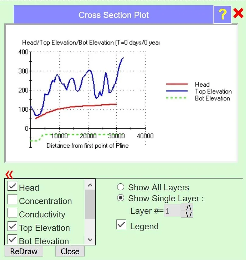
Out of the box, the base model sets the aquifer bottom to the minimum DEM in the domain, offset downward by a constant Z (typically around 100 ft ≈ 30 m) — enough to keep the aquifer a few tens of meters thick everywhere, regardless of topographic relief. This is rarely the most physically accurate choice — real aquifer bottoms follow bedrock, which undulates independently of ground surface. So why is this the default?
If the default used a bedrock raster, there would be places where the bedrock rises close to — or above — the ground surface. Those cells would be dry at startup. A dry cell has zero transmissivity, so the solver can't move water through it, so heads near dry cells can swing wildly or diverge. Result: the model crashes, you see nothing, and you face hours of blind debugging. The "minimum DEM minus constant" default guarantees the aquifer has thickness everywhere, so the solver always finds a solution. That solution is approximate — but you can see it, understand your system, and refine toward accuracy from there. In reality, where bedrock rises to near surface the aquifer may not actually be dry because local K is very small — the robust default is a reasonable realization of that reality.
5.4.2 The customization ladder for bottom
| Rung | Setting | What it gives you |
|---|---|---|
| 0 (default) | Min DEM Minus | Robust flat bottom offset below ground. Always solves. Not physically realistic for most sites. |
| 0 (variant) | Thickness | Bottom = top minus specified thickness. Bottom follows DEM shape (often wrong for flat-lying sediments). |
| 1 | Constant value | Flat bottom at one elevation. Useful for synthetic models; rare for real sites. |
| 2 | Data Center bedrock raster | The big refinement step. In Michigan: "Rock Top Elevation Michigan". Elsewhere: "US Glacial AQ Thickness", "Global AQ Thickness". |
| 3 | Import your raster | Your local bedrock surface — e.g., from local well data or geologic mapping you've processed. |
| 5 (zone only) | Scattered points with interpolation | Discrete borehole measurements interpolated over a zone. |
5.4.3 When to refine from the default
Almost always. For any production modeling, the default bottom is too simple — switching to the Data Center bedrock raster (rung 2) is usually the first refinement you'll make on a new model. It takes one click. The exceptions: synthetic models, teaching demonstrations, or first-look scoping studies where you just want to see what the base flow field looks like on a new domain.
5.5 Hydraulic Conductivity
If you have time to refine exactly one parameter, refine this one. Hydraulic conductivity — K, in meters or feet per day — is the dominant control on flow patterns. It has the full seven-rung customization ladder available.
5.5.1 Why K matters most
Three properties make K the dominant parameter:
- K spans 10 orders of magnitude in natural materials. Gravel ≈ 1,000 m/day. Sand ≈ 10 m/day. Silt ≈ 0.1 m/day. Clay ≈ 0.0001 m/day. Getting K "about right" means getting the right order of magnitude. Getting it "exactly right" is almost impossible — measurements from the same aquifer routinely vary by a factor of 10.
- K scales the entire flow field. Doubling K roughly halves the hydraulic gradient required to drive the same flow. Change K by an order of magnitude and heads change by an order of magnitude. Every refinement you make to K propagates directly into the visualization.
- K couples to every other parameter. Recharge interacts with K to produce heads. Storage interacts with K to determine transient response. Stream leakance interacts with K to determine exchange rates. Refine K and everything else shifts.
5.5.2 The customization ladder for K
| Rung | Setting | Typical use |
|---|---|---|
| 0 (default) | Typical constant (≈22.86 m/day, a sand/gravel value) | Robust starting value for most glacial or alluvial aquifers. Keeps the solver convergent. |
| 1 | Your constant | Your best estimate — ≈10 for sand, ≈100 for gravel, ≈0.1 for silt. |
| 2 | Data Center raster | "Michigan Glacial-Screen to 1st Confining Unit" for Michigan; "GLHYMPS 2.0" globally. Production standard. |
| 3 | Uploaded raster | Your site-specific K field from pump tests, slug tests, or specific-capacity analysis. |
| 5 (zone only) | Scattered points + IDW / Natural Neighbor / Kriging | Discrete well or pump-test K values interpolated over a zone. |
| 6 (zone only) | T-PROGS borehole simulation | Full 3D geologic realization with multiple material types — e.g., 4 materials with K = 53, 5, 0.01, 0.001 ft/day for coarse sand, fine sand, silt, clay. |
5.5.3 Multipliers — the calibration knob
Below the main K field sits a Multiplying Factor. This scales whatever source you've chosen — constant, raster, scattered points, or T-PROGS. A multiplier of 0.3 reduces K to 30% of source values. A multiplier of 1.5 raises K by 50%. Multipliers preserve spatial structure while shifting the overall magnitude, which makes them ideal for calibration.
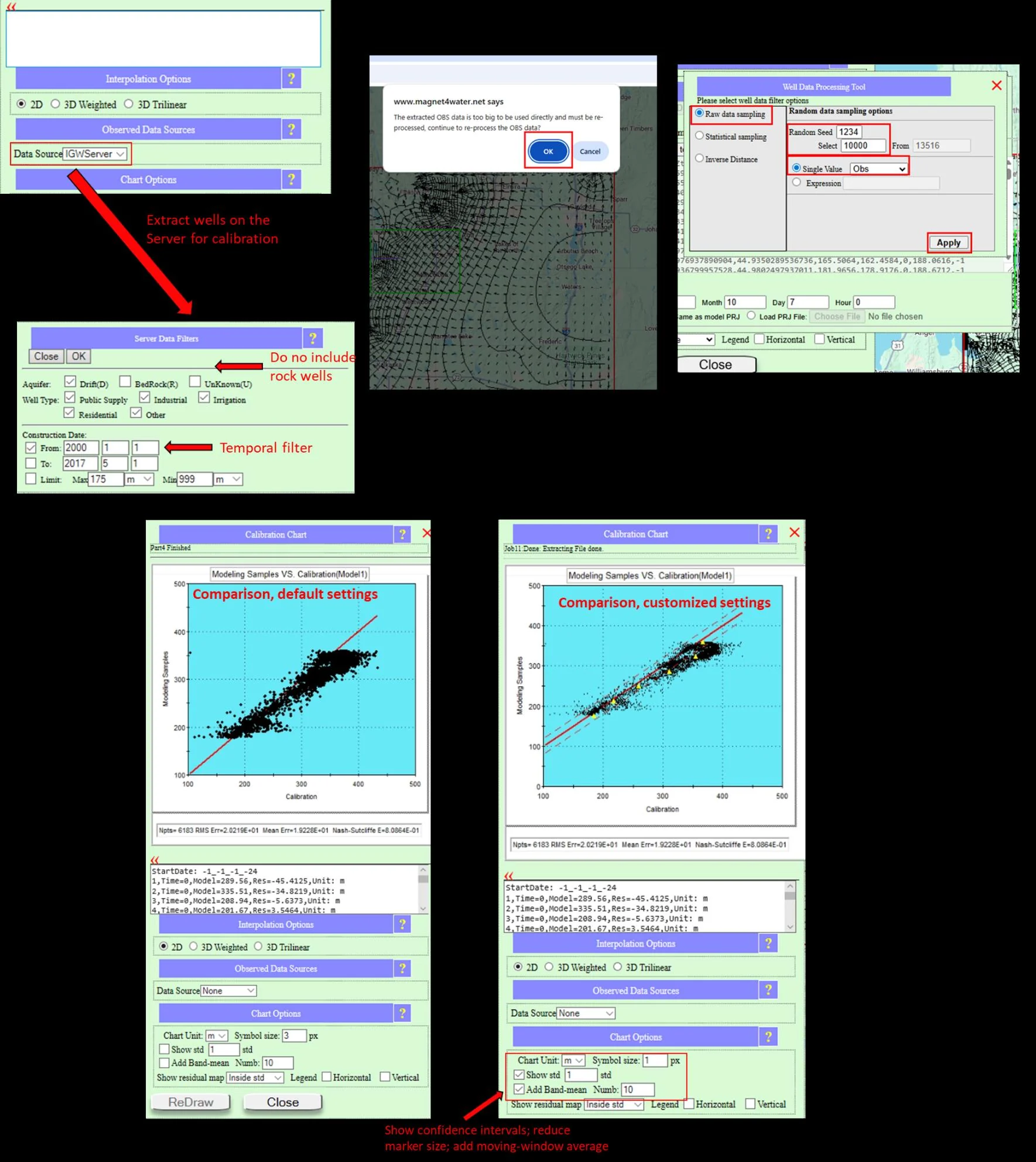
Start with the default, run the model, open the Calibration chart. If heads are systematically too high, simulated flow is too slow — raise K (or lower recharge). If too low, the opposite. Stay within multipliers of 0.3–3.0 on K and 0.5–2.0 on recharge; needing more suggests the problem is structural (wrong bottom, missing feature) rather than parametric.
5.5.4 Why calibrate the multiplier, not the individual cell values
Modelers new to IGW-NET sometimes ask: if the simulated heads don't match observations, why not adjust K cell-by-cell until the match is perfect? Two reasons — one practical, one fundamental.
The practical reason: a K field has thousands of cells. Calibrating each one independently against a few hundred observations is wildly under-constrained. There are infinitely many K distributions that fit observations equally well. Which one is "right"? The process is ill-posed — mathematically unsound.
The fundamental reason: a model fitted that way is not more predictive. It is overfit. It reproduces the observations you had, but fails when the system is stressed in a new way — a new pumping well, a different climate year, a spill at a new location. A predictive model is one whose parameters reflect real physics, not one whose parameters have been tuned to memorize the past.
Consider what happens when you use a Data Center K raster derived from USGS water-well lithologies — one of the most common starting points for real-world modeling. Calibrating the multiplier on that raster (one parameter) almost always shows the multiplier needs to be less than 1.0 — often around 0.3 to 0.5.
This isn't a bug; it's a feature of the data. Water wells are sited where K is high — nobody drills a production well into a clay aquitard. So a raster built from well lithologies is systematically biased toward the high end of the local K distribution. A multiplier of 0.3 on such a raster makes physical sense: it adjusts the whole field to reflect the volume-averaged K, which is what a regional groundwater model actually cares about. The spatial pattern (where K is higher than where) stays intact; only the overall level shifts.
This is what makes multiplier-based calibration defensible: the multiplier has a physical meaning you can interpret. Individual-cell calibration does not. When in doubt, calibrate the multiplier and leave the raster pattern alone.
5.5.5 Anisotropy — Kxx/Kyy and Kxx/Kzz
Real aquifers rarely conduct water equally in all directions. IGW-NET captures this with two anisotropy ratio fields:
- Kxx/Kyy: horizontal ratio, default 1.0 (isotropic in plan view). Rarely changed.
- Kxx/Kzz: vertical ratio, default 10.0 (horizontal K is 10× vertical K). Reasonable for typical layered sediments; raise to 50+ for strongly laminated silty aquifers, lower to 1–3 for clean sands.
Vertical anisotropy matters mostly for systems with significant vertical flow — pumping wells drawing from multiple layers, recharge migrating down, lakes exchanging water with deep aquifer. For purely horizontal regional flow, the default is usually fine.
5.6 Porosity and Storage
Three values under the Storage Coefficients heading. Each has a typical default set for numerical robustness; each becomes important in specific contexts.
| Parameter | Default | Typical range | Used for |
|---|---|---|---|
| Specific Yield (Sy) | 0.1 | 0.05 – 0.25 | Transient unconfined flow. Ignored for steady-state. Ignored for confined aquifers. |
| Specific Storage (Ss) | 10⁻⁵ per meter | 10⁻⁶ – 10⁻⁵ per meter | Transient confined flow. Much smaller than Sy. Only matters when Sy doesn't apply. |
| Effective Porosity | 0.3 | 0.2 – 0.35 | Transport and particle tracking. Controls advection velocity. Not used for flow. |
5.6.1 Refinement ladder
These three fields offer fewer rungs than K. Typical refinement goes:
- Rung 0 (default): 0.1, 10⁻⁵, 0.3. Numerically robust, physically reasonable for typical sand aquifers.
- Rung 1 (your constants): Replace with site-appropriate values — e.g., Sy=0.2 for clean sands, Sy=0.05 for silty aquifers, porosity=0.25 for moderately packed sediment.
- Rung 5 (zone-only, scattered points): For detailed investigations where you have discrete measurements at specific locations, scattered-point interpolation is available at the zone level.
For steady-state flow: none of these matter — defaults are fine, the solver ignores them. For transient flow: Sy (or Ss for confined) matters a lot; getting it wrong changes how fast the aquifer responds to stress. For transport or particle tracking: effective porosity matters a lot — a porosity of 0.3 moves plumes 33% slower than a porosity of 0.2.
5.7 Recharge
The second major water input, alongside any lateral inflow from boundaries. Recharge is the rate at which precipitation becomes groundwater after surface runoff and evapotranspiration.
5.7.1 Customization ladder
| Rung | Setting | Typical use |
|---|---|---|
| 0 (default) | Typical constant — around 15 inch/year (~380 mm/year) | Humid-region starting value. Works immediately for most US/EU sites. |
| 1 | Your constant | Adjust to your climate — 5 inch/year for semi-arid, 25+ for tropical wet seasons. |
| 2 | Data Center raster | "Global w/MI Patch" — globally available with Michigan high-res inset. USA alternative: "USA Long-term Mean (USGS)". |
| 3 | Uploaded raster | Site-specific recharge map from detailed water-balance analysis. |
| 4 | DataNET WFS/WCS | Dynamic precipitation service for long-term monitoring applications. |
| — (advanced) | From Watershed Solver output | When the Watershed Solver runs and computes infiltration; its output then feeds groundwater recharge. See Chapter 15. |
5.7.2 Typical values by climate
| Climate / setting | Typical annual recharge |
|---|---|
| Great Lakes region (MI, OH, WI, MN) | 10–20 inch/year (250–500 mm/year) |
| Humid southeast USA | 8–18 inch/year |
| Semi-arid western USA, irrigated | 2–6 inch/year |
| Arid / desert | 0–1 inch/year |
| Tropical wet season | 20–40 inch/year, highly seasonal |
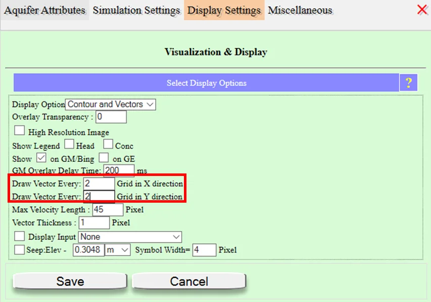
The recharge field's unit dropdown defaults to inch/year. If you type 50 thinking you're entering millimeters per year, the solver sees 50 inch/year — wildly wet, flooding the domain. Always glance at the unit dropdown before typing.
5.8 Surface Drainage — the Quiet Workhorse
Of all seven attributes, this is the one that most users never notice — and the one that most shapes how realistic their model looks.
5.8.1 What it does
In nature, when groundwater rises to ground surface, it does not keep rising. It seeps out — as springs, wetlands, seeps, riparian zones, or inflow to streams. IGW-NET represents this without requiring you to draw every seep as a feature: every cell in the domain is treated as a potential surface drain. When the simulated head rises above the ground surface at that cell, water discharges from the aquifer at a rate proportional to the excess head times the surface drainage leakance.
At any cell where h > zsurface:
Qdrain = (h − zsurface) × leakancesurface
When h ≤ zsurface: no drainage. The aquifer is below ground, as expected.
The default surface-drainage leakance is 1/day, active by default. You rarely need to change it.
5.8.2 Why this is a superpower
The ground surface from a modern DEM is rich with information. Rivers sit in valleys. Lakes occupy local depressions. Wetlands occupy flat areas where the water table approaches the surface. When the surface drain is active:
- Your simulated head rises to the ground surface in the right places — where rivers, lakes, and wetlands actually exist.
- The drain sheds the excess, simulating natural discharge without you drawing anything.
- Flow patterns match topographically-controlled reality. Groundwater flows from highlands toward valleys, converges on major rivers, disperses into wetlands.
In most sites, DEM-based surface drainage captures 90%+ of how surface water controls groundwater. Rivers, lakes, and wetlands exist where they do because of topography — and the DEM knows the topography. The single most important thing you can do to make a model look realistic is simply leave this default on. How rivers bend, where big lakes sit, where wetlands appear — all of it is encoded in the DEM, and the surface drain translates it directly into the flow field.
5.8.3 When to refine to explicit rivers and lakes
DEM-as-drain is one-way. Water can leave the aquifer through surface drainage, but water cannot enter the aquifer from surface water. For most regional modeling this is fine — the dominant effect of surface water is to drain groundwater. But sometimes surface water recharges groundwater: losing streams in arid regions, lakes in glacial depressions, leaking reservoirs, rivers where the water table is deeper than the streambed.
The one-way default is rooted in a simple mass-balance truth: in a regional area with non-trivial recharge, whatever comes down has to go up. Precipitation infiltrates over a broad area; that water has to leave the aquifer somewhere. Over regional scales in humid and temperate climates, the dominant exit is discharge to surface water — rivers, lakes, wetlands, springs. Surface water functions as a drain for the groundwater system because it has to. Treating SW this way automatically produces a globally consistent water balance.
Arid and semi-arid regions can break this assumption. Where the water table is deep and surface water is scarce — arroyos that run only after storms, isolated playas, ephemeral lakes — the regional flow system may not be connected to surface water in the usual way. In these settings, losing streams and episodic infiltration from surface water can be important. Even there, if you model a large enough area, the mass-balance logic eventually takes over. But for site-scale or basin-scale modeling in arid regions, explicit two-way features may be appropriate from the start.
Beyond the mass-balance argument, there is a practical reason: misconfigured two-way boundaries are one of the easiest ways to silently break a model's water balance. A two-way feature requires careful specification — stage, conductance, geometry — and when any of these is off, you can get flow patterns that look plausible while the water balance is wildly wrong. Surface water inadvertently flooding the aquifer through a misconfigured lake, or a river acting as an effectively infinite source, can produce heads that contour nicely but are fundamentally meaningless. The one-way default trades a small amount of physical realism for large insurance against a failure mode that is hard to detect.
None of this is locked in. IGW-NET is designed so that every conceptual-model assumption is editable, and every edit is immediately reflected in the visualization. If the one-way default doesn't fit your system, you change it — draw explicit rivers and lakes, set them as two-way head-dependent, re-simulate, and watch how the flow field and water balance respond. The platform is less a calculator than a visual sandbox for your thinking: every conceptual choice you make becomes a visible outcome you can check against reality and intuition.
When two-way exchange matters and you have the physical understanding to configure it correctly, you move to explicit features — line features for rivers and drains, polygon features for lakes and wetlands. This is Chapter 6's subject. A preview of how IGW-NET configures these automatically:
| Feature | Default treatment (DEM-as-drain) | Explicit refinement |
|---|---|---|
| Small rivers (1st–2nd order) | Captured by DEM-as-drain | Drawn as one-way drain line features. |
| Larger rivers (3rd order and above) | Captured by DEM-as-drain | Drawn as two-way head-dependent line features. GW ↔ SW exchange both directions. |
| Small lakes / ponds | Captured by DEM-as-drain | Drawn as one-way drain polygon features. |
| Larger lakes | Captured by DEM-as-drain | Drawn as two-way head-dependent polygons, optionally with bathymetry and coupled stage. |
5.8.4 Leakance for explicit features — the physics
When you add explicit rivers and lakes, each one has its own leakance — and here the units diverge in a way that often confuses new users. The reason is physics, not UI quirk.
leakanceriver = (Ksediment / thicknesssediment) × widthchannel
A line has no intrinsic width, so the channel width enters explicitly. The result has units of m/day (flux per unit length of line). Typical river leakance: 1–10 m/day for ordinary streambeds.
leakancelake = Ksediment / thicknesssediment
A polygon already has area, so no width factor. The result has units of 1/day (flux per unit area). Typical lake-bed leakance: 0.01–1/day; reservoirs with leaky bottoms up to 5/day; boundary-condition polygons that should behave as prescribed head can use 5,000/day to effectively enforce the specified stage.
Both forms represent the same underlying quantity — the hydraulic conductance of the bed sediment. They differ because a line is integrated over the channel width while a polygon is integrated over its own area. One extra dimension, different units. Once you see why, the "different units" question stops being confusing.
5.9 The Defaults — All In One Place
Every parameter the base model relies on, its default value, and why that default was chosen. If you remember only one table from this chapter, make it this one — it is what makes the base model work.
| Attribute | Default value | Reason for the default |
|---|---|---|
| Top elevation | DEM (auto-matched to grid) | DEM is always the right answer for real sites. Auto-matching picks the resolution that makes sense for the cell size. |
| Bottom elevation | Min DEM minus constant | Guarantees aquifer thickness everywhere → no dry cells → solver always converges → you always see a solution. |
| Hydraulic conductivity | ≈22.86 m/day (sand aquifer) | Typical of glacial sand and gravel — the most common surficial aquifer in many regions. Gives reasonable initial flow. |
| Kxx/Kyy ratio | 1.0 | Horizontal isotropy is the default assumption for regional modeling. Rarely worth changing. |
| Kxx/Kzz ratio | 10.0 | Typical layered sediments conduct horizontally ~10× more than vertically. Good starting estimate. |
| Specific Yield (Sy) | 0.1 | Midrange unconfined-aquifer value. Numerically stable for transient simulations. |
| Specific Storage (Ss) | 10⁻⁵ per meter | Typical elastic-compression value. Correct order of magnitude for confined aquifers. |
| Effective Porosity | 0.3 | Typical sand/gravel effective porosity. Matters only for transport and particle tracking. |
| Rain recharge | ≈15 inch/year | Humid-temperate starting value. Realistic for eastern US, Great Lakes region; refine for other climates. |
| Surface drain leakance | 1/day (active) | Typical effective rate for near-surface sediments. Shedding excess head produces realistic drainage patterns. |
| Starting head | Top elevation (water table at surface) | Most wet starting guess. Ensures cells start saturated so the solver has a valid initial field. |
5.9.1 When to think about each default
Not all defaults are created equal. Some are fine forever; some demand early attention. Here's the priority order most modelers follow:
- Refine first: Bottom elevation (to Data Center bedrock), hydraulic conductivity (to Data Center raster), recharge (to Data Center).
- Refine next, if transport or transient: Specific yield (for transient unconfined), effective porosity (for transport).
- Refine rarely: Kxx/Kyy, Kxx/Kzz, surface drain leakance, starting head.
5.10 Zones: Refinement With Teeth
Everything you have learned about aquifer attributes applies to the whole domain. A parallel dialog — the Zone Attributes window — lets you override all of it inside any polygon you draw. Zones are how you refine locally without rebuilding.
5.10.1 The zone–domain precedence rule
The rule is simple and consequential: where a zone is defined, the zone's attribute values take precedence over the domain's background values. Where the zone is silent, the domain fills in.
This means you can draw a zone covering 10% of your domain, specify only K inside that zone, and leave every other attribute unset — the zone will use its own K but the domain's top, bottom, recharge, porosity, storage, and drain leakance. Zones are additive and selective; they refine what you want and inherit the rest.
5.10.2 What zones add beyond the domain
Zones are not just "a domain in a smaller area." They unlock refinement options that the domain alone does not offer:
| Refinement | Domain | Zone |
|---|---|---|
| Typical defaults (rung 0) | Yes | Yes (inherits from domain) |
| Your constant (rung 1) | Yes | Yes |
| Data Center raster (rung 2) | Yes | Yes |
| Uploaded raster (rung 3) | Yes | Yes |
| DataNET service (rung 4) | Yes | Yes |
| Scattered points + interpolation (rung 5) | — | Yes (IDW, Natural Neighbor, Kriging) |
| T-PROGS borehole simulation (rung 6) | — | Yes (K only) |
Scattered-point interpolation and T-PROGS exist at the zone level because they are inherently local — you have measurements at specific points in a specific area. Applying them to the whole domain rarely makes sense; applying them to the zone around a site investigation does.
5.10.3 The submodel — instant local refinement
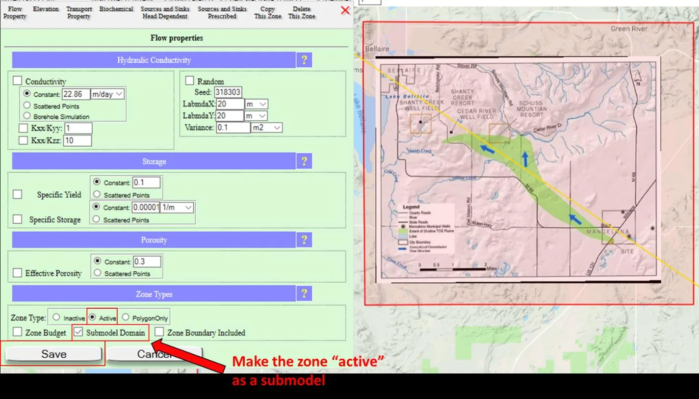
A special kind of zone — the Submodel Domain — takes refinement further. You draw a box inside the parent domain, check Submodel Domain → Active in the Zone Attributes menu, and check Boundary Condition from Parent Model in the Simulation Settings of Domain Attributes. That's it. You have a refined, smaller-area model whose boundary conditions are automatically inherited from the parent's head solution.
Start regional and coarse. Run. See where detail matters — near a well field, near a contamination source, at a site investigation. Draw a submodel box around that area. One click: "Boundary Conditions from Parent Model." Re-simulate. You now have a refined local model with correct regional context. Total time: about a minute. This workflow — regional-to-local nesting with inherited BCs — is what makes incremental modeling in IGW-NET virtually instantaneous. See Chapter 13 for the full treatment.
5.10.4 A three-layered mental model
As you refine, your model accumulates three layers of attribute specification:
- Domain defaults — what applies everywhere unless overridden.
- Zone overrides — what applies inside zone polygons.
- Submodel (also a zone) — a special zone type whose boundary conditions come from the parent.
Everything else in IGW-NET — line features, wells, particle zones, transport sources — layers on top of these. Master the three aquifer-attribute layers and you have the conceptual foundation for everything that follows.
5.11 Seeing Your Current Approximation
Every model you run in IGW-NET is a visualization of your current approximation — not of reality. As you refine attributes and add features, the visualization shifts toward reality. Learning to read the gap between them is the fastest path to skilled modeling.
5.11.1 What the visualization reveals
Every output of the base model tells you something about what your current attributes imply. Read each output as a question — and let the answer guide your next refinement.
| Output | What it's telling you | What to refine if it looks wrong |
|---|---|---|
| Head contour pattern | How groundwater is moving at regional scale | K distribution; boundary conditions; recharge |
| Head magnitude vs. observations | Whether your flow system produces the right water levels | K × multiplier; recharge × multiplier |
| Velocity vector density | Where flow is fast vs. slow | K heterogeneity; stream features; pumping patterns |
| Seepage / drainage zones | Where groundwater emerges at surface (wetlands, springs) | Usually fine with defaults; add explicit streams if two-way exchange matters |
| Cross-section head vs. bottom | Is the aquifer thick everywhere, or going dry somewhere? | Bottom elevation from default to Data Center bedrock |
| Plume / particle trajectory | Where water actually goes — the integrated flow field | K distribution (especially vertical heterogeneity — layers or T-PROGS) |
| Water balance | Whether all inflows and outflows balance sensibly | Boundary conditions; recharge; drain leakance |
5.11.2 Incremental modeling in practice
The philosophy underlying this entire chapter: you build understanding by refining in small steps, not by assembling a "correct" model in one shot. Starting complex is a pitfall — when something goes wrong, you won't know where. Starting simple and refining gives you a chain of working models, each one a baseline for the next, each one showing you what the last refinement changed.
- Start coarse and simple. Relatively coarse grid, 2D, one conceptual layer, all domain defaults. Run. Look at the base flow field. Resist the urge to add complexity before you see what simple gives you.
- Refine the biggest lever first. Usually that's bottom elevation and K — switch both to Data Center. Re-run. Compare.
- Check against observations. If you have water-level data, open the Calibration chart. Adjust multipliers (not individual cell values) if the bias is obvious.
- Let sensitivity analysis tell you what matters. IGW-NET's real-time sensitivity analysis reveals which parameters actually move the answer — and which don't. Refine the sensitive ones. Leave the insensitive ones at their defaults.
- Add vertical detail only if sensitivity demands it. If the cross-section looks adequate with one layer and vertical parameters don't show up as sensitive, keep it simple. If vertical flow matters (pumping, lakes), then add sublayers or conceptual layers.
- Use submodels for local refinement. Don't refine the whole domain — refine where detail matters. Draw a box, check "parent BC," one click. You have a detailed local model with correct regional context.
- Add transport and particles when you have a flow field you trust. The transport and particle patterns then become a second check on the flow field itself — they reveal how water integrates over time, which is often more revealing than heads alone.
- Stop refining when data can't justify more complexity. An elaborate K field that calibrates beautifully against sparse observations is not a better model. It is an ill-posed exercise that produces worse predictions than a simpler, better-constrained alternative. Simplicity is a feature.
Every step is a short loop: refine → run → visualize → decide. No refinement is "all or nothing." You can always go back. And when something looks wrong, you know which change caused it, because you only made one at a time.
5.11.3 The insight is the product
It is tempting to think of a model as an equation-solving exercise that produces a prediction. That framing misses the point. Modeling in IGW-NET is a sense-making exercise: the base model gives you a first look, each refinement sharpens the picture, and somewhere along the way you develop genuine understanding of how your system works — which processes dominate, which parameters are most sensitive, where the flow actually goes.
Calibration and prediction come after that understanding, not before. They become possible — and defensible — because you have walked up the customization ladder thoughtfully, stopped where data and sensitivity analysis no longer justified more complexity, and seen how each refinement shifted the visualization. A defensible simple model that you understand beats a complex model that calibrates well but hides its own assumptions. Insight is the real product of modeling. The platform is designed to get you there as fast as possible — and to stop you from going further than you should.
Underneath all of this sits a simpler design principle: every conceptual assumption in your model is editable, and every edit is immediately visualized. None of the defaults are locked in. You can change the aquifer bottom, switch K from constant to raster to T-PROGS, toggle DEM-as-drain for explicit two-way rivers, redraw domain or submodel, add layers, add sources — and each change produces a new visible result you can judge. This is what makes IGW-NET less a calculator than a visual sandbox for your thinking. The model is not an artifact you build and hand off. It is a living representation of your current understanding, and every question you have about your system is one edit and one simulation away from an answer.
To go deeper
- Quick Tutorial 1: 2D Steady Flow — hands-on walkthrough of the base model covered here.
- Quick Tutorial 2: Nested Modeling — the submodel workflow demonstrated step-by-step.
- Quick Tutorial 8: Calibration — the practice behind §5.5.4's discussion of multipliers vs. individual-cell calibration.
- Quick Tutorial 19: Auto Parameter Estimation — automated calibration while preserving spatial structure.
- Quick Tutorial 24: T-PROGS 3D Geologic Model — the top rung of the ladder for hydraulic conductivity.
- Platform Concept: Fallback vs Spatial Values — deep dive on Data Center rasters.
- Platform Concept: Surface Drainage as Wetland Predictor — the full story behind §5.8.
- Pinder Beginner's Manual, §3.2 — the academic-style treatment with more hydrogeology context.
- Case Study: Mancelona TCE Plume — the customization ladder in action at a real Michigan site.
- Case Study: Barron Lake Coupled Model — two-way lake coupling and T-PROGS in a production context.
- Platform Reference: hydraulic_conductivity — the underlying schema for K and its encoding.