The quick read — 90 seconds
- Stochastic modeling in IGW-NET includes both single-realization and ensemble analyses. Single realization: one random field, one simulation, showing how heterogeneity affects flow. Ensemble: many realizations with aggregated statistics for uncertainty quantification. Both are legitimate stochastic work.
- Spatially correlated random fields are the unifying framework. Sequential Gaussian Simulation (SGS) handles continuous variables (K, porosity, recharge, retardation, elevations); T-PROGS (Ch. 17) handles categorical materials. Same conceptual framework, two methods.
- Any spatial input can be randomized. K, effective porosity, water density, recharge, partitioning Kd (retardation), top/bottom elevations, layer thickness. Per-zone configuration with correlation scales (LambdaX/Y/Z), mean, variance, seed, nugget, anisotropy angles.
- Single realization shows realistic flow structure. Head contours distort around low-K zones; flow vectors bend and channel; particle paths become tortuous and asymmetric. One realization visualizes what heterogeneity actually does — a powerful teaching and client-communication tool without any ensemble.
- Monte Carlo ensemble produces probabilistic outputs. Many realizations feed recursive ensemble statistics. Outputs: mean head field, head variance map, probability distributions at monitoring wells, probabilistic capture zones.
- The recursive-statistics architecture is the distinctive IGW-NET innovation. Running mean and variance are updated per realization using Welford's algorithm; the ensemble is never stored. Memory cost: O(cells × statistics types), not O(cells × realizations). Run 10 realizations or 10,000 with the same memory footprint. Compute-render-discard — same pattern as IGW-NET transient visualization.
- Ensemble smooths as realizations accumulate. Watch the mean head field visibly refine with each new realization; the variance map stabilizes; probability distributions populate. Real-time feedback on ensemble convergence — you can stop when statistics have converged rather than predetermining a fixed count.
- Macrodispersion is the excess spreading of the mean plume beyond any single realization's plume — a fundamental heterogeneity effect not capturable by uniform-K or smoothly-varying K models.
- Probabilistic capture zones express the capture region as a probability field rather than a hard boundary — essential for risk-based wellhead protection and contaminant source management.
- Stochastic analysis quantifies parameter uncertainty, not structural uncertainty. Monte Carlo ensembles on structurally-flawed models give confidence intervals that exclude the correct answer. Structure-first (Ch. 18 §18.1.3) still applies — stochastic modeling refines a sound model; it cannot rescue a flawed one.
19.1 What Stochastic Modeling Is — Single Realizations and Ensembles
Stochastic modeling in groundwater practice covers a broader territory than Monte Carlo simulation alone. Both single-realization analysis and ensemble simulation belong here; IGW-NET supports both.
19.1.1 The two forms of stochastic analysis
Two kinds of stochastic work address different questions:
| Form | What you do | Question it answers |
|---|---|---|
| Single-realization simulation | Generate one spatially correlated random field (K, recharge, or another variable); simulate flow and transport through it once | "What does heterogeneity do to the flow and transport solution?" Shows realistic tortuous flow paths, channeled high-K flow, preferential transport — what you cannot see with uniform-K modeling |
| Ensemble Monte Carlo simulation | Generate many realizations (tens to thousands); simulate each; compute ensemble statistics (mean, variance, probability distributions) | "How uncertain is the answer?" Produces probabilistic outputs: mean heads, variance maps, confidence intervals on fluxes, probabilistic capture zones |
These are both stochastic analyses — both treat spatial inputs as random variables. Single-realization shows the effect of randomness (the qualitative structure of heterogeneous flow); ensemble quantifies uncertainty under that randomness (the quantitative spread of possible outcomes). Many projects benefit from both: start with a single realization to understand heterogeneity effects; escalate to ensemble when uncertainty quantification is needed.
19.1.2 Why single-realization is valuable on its own
A common misconception: "stochastic modeling requires many realizations." Not always. A single well-chosen realization can be a valuable analysis by itself:
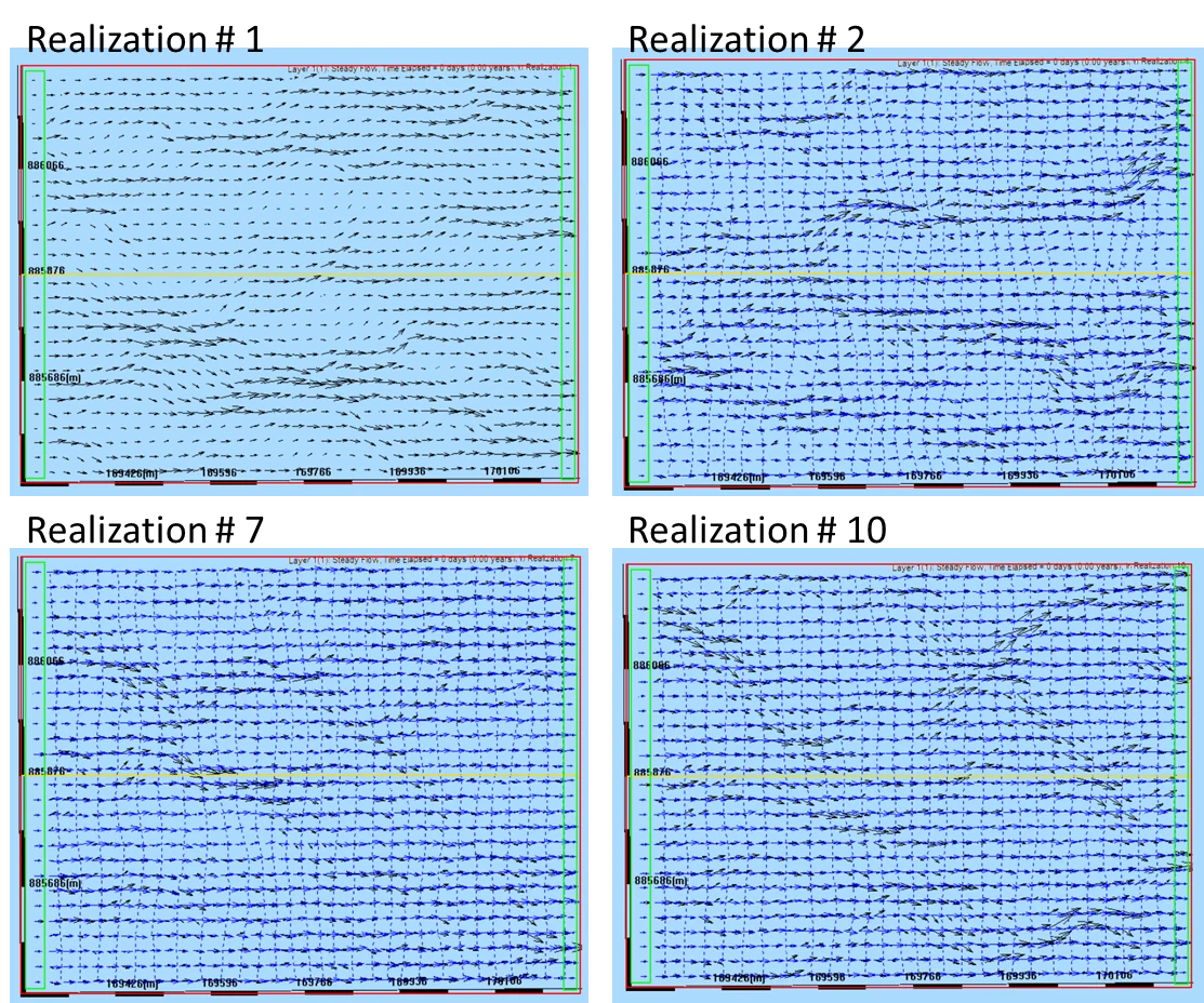
- It shows realistic flow physics. Head contours distort around low-K zones; flow vectors bend and channel through high-K corridors; particle paths twist and diverge rather than following smooth uniform-K trajectories. These are visual features of real aquifers that uniform-K models systematically miss.
- It teaches the role of heterogeneity. For students, clients, or collaborators unfamiliar with groundwater heterogeneity, a single realization is the most direct demonstration. "This is what your aquifer actually looks like, roughly, in terms of its flow structure. This is why smooth-K predictions can be misleading." Synthetic mode (Ch. 1 §1.3.2) is especially effective here — enter it via Utilities → Go to Synthetic Case Area, and you can toggle heterogeneity on and off with a single click, watching the dramatic effect of K structure on transport immediately, without real-site complications obscuring the lesson. The emergence of macrodispersion from small-scale heterogeneity — the nonlinear scale effect — is vivid right in front of the class. Work through Tutorial 15 (Single-Realization Stochastic Flow) and Tutorial 17 (MC Transport) for the full recipe.
- It is one hypothesis — useful in its own right. The real K field in the ground is unknown; a realization is one physically-plausible arrangement consistent with the available statistics. For planning, design, or "what if the aquifer is like this?" questions, one realistic hypothesis often does what a full ensemble would.
- It can be run quickly. A single realization costs essentially what a single deterministic simulation costs — no ensemble overhead. For exploratory work, this is the right level of effort.
Move to ensemble Monte Carlo when the question specifically requires uncertainty quantification — probabilistic capture zones, breakthrough curve distributions, confidence bounds for risk-based decisions. Don't run an ensemble when a single realization would answer your question.
19.1.3 What the rest of this chapter covers
Section 19.2 establishes spatially correlated random fields as the conceptual framework uniting SGS (continuous) and T-PROGS (categorical). Section 19.3 covers SGS setup in detail: which variables can be randomized, what parameters govern the random field, how per-zone configuration works. Section 19.4 walks through single-realization analysis. Section 19.5 covers the full ensemble Monte Carlo workflow. Section 19.6 is the distinctive IGW-NET contribution: the recursive ensemble-statistics architecture that makes arbitrary realization counts feasible at full model resolution. Section 19.7 covers result interpretation — mean fields, variance maps, probability distributions, macrodispersion, probabilistic capture zones. Section 19.8 connects back to calibration (Ch. 18) for parameter uncertainty as stochastic input. Section 19.9 collects common pitfalls, including the critical one that stochastic analysis does not quantify structural uncertainty.
19.2 Spatially Correlated Random Fields — The Unifying Framework
IGW-NET's two main stochastic methods — Sequential Gaussian Simulation (this chapter) and T-PROGS transition probability (Ch. 17) — are different operational techniques within a common conceptual framework: both produce spatially correlated random fields. Understanding the framework helps clarify when to use which method.
19.2.1 What "spatially correlated random field" means
A spatially correlated random field is a collection of values, one at each cell in the domain, with two key properties:
- Random. Values are drawn from probability distributions, not prescribed deterministically. Running the generation with different random seeds produces different-looking fields.
- Spatially correlated. Neighboring cell values are not independent — they're related through a specified correlation structure. Cells within the correlation scale tend to have similar values; cells beyond the correlation scale are effectively independent.
The correlation structure is what makes the field "realistic." Completely independent random values at every cell would produce pure noise — a salt-and-pepper pattern with no geological meaning. Real aquifers don't look like that. They have regions of high-K sand grading to regions of low-K clay, with characteristic length scales (the correlation scale) determined by depositional processes. The correlation structure in the random field captures that reality.
19.2.2 Continuous vs. categorical random fields
Two fundamental types of spatially correlated random fields:
| Type | What's random | Method in IGW-NET | When appropriate |
|---|---|---|---|
| Continuous | A continuous numerical value (K, log K, porosity, recharge rate) | Sequential Gaussian Simulation (SGS) — §19.3 | When the variable is naturally continuous — gradual variations in alluvial deposits, smooth variations in recharge, porosity variation within a single lithology |
| Categorical | A discrete category (AQ, MAQ, PCM, CM — aquifer material classes) | T-PROGS — see Ch. 17 | When the spatial pattern is layered, with sharp contacts between distinct materials — glacial stratigraphy, stratified sedimentary systems, any layered aquifer |
SGS and T-PROGS aren't competing methods; they're appropriate for different kinds of heterogeneity. A sandy aquifer with continuous variation of grain size (affecting K smoothly) is SGS's natural territory. A layered glacial aquifer with discrete sand, silt, and till units is T-PROGS's natural territory. Some sites benefit from both: T-PROGS for the layered structural framework (where the main AQ/CM contacts are) plus SGS within each unit for the continuous variation (K variation within the sand layer). IGW-NET supports mixing them through the zone-level configuration.
19.2.3 The common workflow pattern
Both methods share the same high-level operational pattern:
Specify the statistical structure
For SGS: mean, variance, correlation scales, variogram type. For T-PROGS: material categories and transition probabilities (typically estimated from borehole data). Both capture how the field varies in space.
Generate one or more realizations
Each realization is one specific random arrangement consistent with the statistics. A seed controls the random number generator; same seed = same realization, different seed = different realization.
Simulate flow (and transport, particles, etc.) through the realization
The random field becomes the model's K field (or porosity, recharge, etc.). Standard simulation proceeds from there.
Analyze — either the single realization, or ensemble statistics
For single-realization analysis: examine the resulting flow structure directly. For ensemble: accumulate statistics across many realizations.
From §19.3 onward, the focus is on SGS specifically. T-PROGS is covered in its own chapter (Ch. 17). Where appropriate, ensemble-statistics sections apply to both methods identically.
19.3 Sequential Gaussian Simulation — Continuous Random Fields
Sequential Gaussian Simulation (SGS) is the standard geostatistical method for generating continuous random fields. IGW-NET supports SGS for any continuous spatial input variable — K is the most common use, but porosity, recharge, retardation, and elevations are equally valid.
19.3.1 Which variables can be random fields
In IGW-NET's zone-level configuration, any of these variables can be flagged as random:
| Variable | Typical use case |
|---|---|
| K (hydraulic conductivity) | The most common random field. Represents aquifer heterogeneity for flow and transport. |
| Effective Porosity | Affects groundwater velocity (v = q/n); matters for transport travel times. Typically more tightly constrained than K but still has real variability. |
| Water Density | For variable-density flow problems (coastal interface, brines). Random density captures uncertainty in salinity distribution. |
| Recharge | Spatially variable recharge uncertainty — different land cover, soil types, climate variability creating a range of possible recharge patterns. |
| Partitioning Kd (retardation factor) | For reactive transport; Kd heterogeneity produces preferential retardation pathways. Essential for realistic contaminant transport predictions. |
| Top Elevation | Aquifer top uncertainty — particularly relevant for confined systems where the top of the aquifer controls head. |
| Bottom Elevation | Bedrock surface uncertainty — particularly relevant where bedrock depth varies and is known only at scattered borehole locations. |
| Thickness | Layer thickness variability — for layered systems where the geometry itself is uncertain. |
Each zone can independently configure which of these are random. A common setup: K random everywhere; porosity random in the AQ zone only (where it matters most for transport); elevations deterministic from the Data Center. Flexibility matches the geological and hydrologic reality of the site.
19.3.2 The random field parameters
Each random field is specified by a small set of statistical parameters, configured per-zone-per-variable:
| Parameter | What it controls | Typical values (for K) |
|---|---|---|
| Mean | The average value of the field (or of log K for lognormal distributions) | The zone's nominal K — e.g. 10 ft/day for a sandy aquifer zone |
| Variance | How spread out the values are. Higher variance = more extreme high and low values | For log K: 1–4 (K spans 1–2 orders of magnitude around the mean) |
| LambdaX, LambdaY | Correlation scales in X and Y directions. Points closer than Lambda are correlated; beyond Lambda, effectively independent | Horizontal: 100–1000 m typical for sedimentary aquifers; reflects depositional layer lengths |
| LambdaZ | Correlation scale in Z direction. Usually much smaller than LambdaX, reflecting thinner layering vertically | Vertical: 1–10 m typical; 10–100× smaller than horizontal correlation |
| Seed | Random number generator seed. Same seed = same realization; controls reproducibility | Any integer; user-selectable for reproducible results |
| Nugget | "Pure noise" component added to the correlated field — reflects sub-grid heterogeneity or measurement noise | Typically 0 or a small fraction of variance |
| Anisotropy angles (AngleX, Y, Z) | Rotation of the correlation ellipse relative to model axes — for tilted geological fabrics | Typically 0 (axes aligned with model grid) |
19.3.3 The correlation-scale choice matters
Of all the parameters, the correlation scale (Lambda) is the most impactful on model behavior and the most often misconfigured. Small LambdaX (say 10 m in a 10-km model) gives near-independent noise — salt-and-pepper heterogeneity that doesn't look like geology. Very large LambdaX (say 10 km in a 10-km model) gives fields that are essentially constant across the domain — not much heterogeneity at all.
Think about the geological unit being represented: what is the characteristic length of a single "body" in that unit? For glacial outwash, it's the length of a typical outwash body — maybe 100-500 m. For alluvial sand, the length of a channel belt — maybe 200-2000 m. For loess or uniform eolian deposits, larger (1-10 km). Vertical correlation scales follow layer thicknesses — 1-10 m for most sedimentary systems. The Data Center can provide typical correlation scales for standard geologic settings; literature reviews (e.g., Gelhar's compilation, or aquifer-specific studies) give published ranges. Using the zone's nominal geological setting to guide LambdaX, Y, Z is much better than generic defaults.
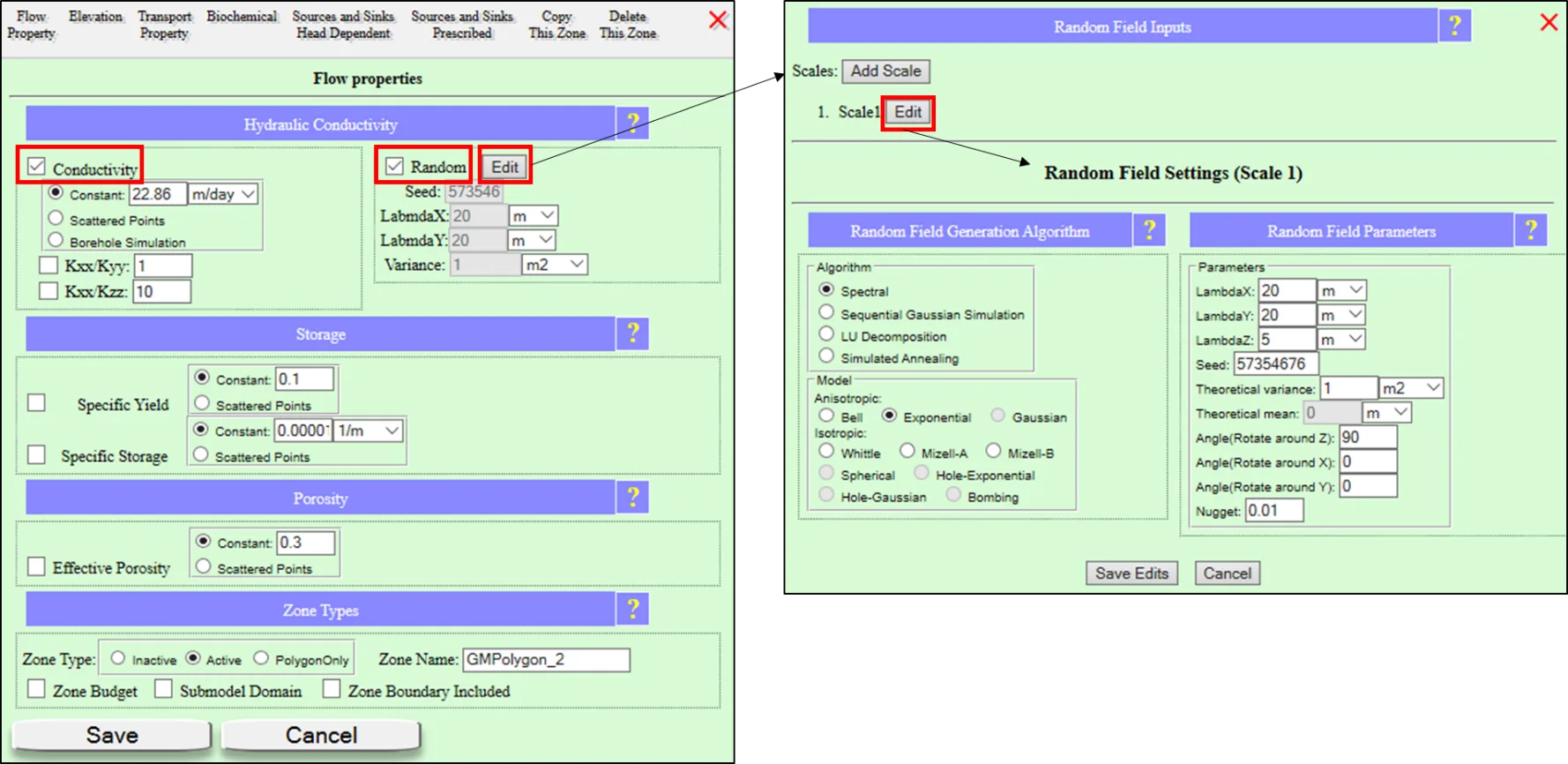
19.3.4 Log-normal vs. normal K
Hydraulic conductivity is conventionally modeled as lognormally distributed — log K is Gaussian, K itself is lognormal. This matches empirical observation: K in natural aquifers spans many orders of magnitude, with values clustered in the middle of log space and tails extending to very high and very low values. SGS in IGW-NET operates on log K by default for hydraulic conductivity, converting to K via exponentiation for the flow simulation. The Mean and Variance parameters, for K, refer to the log-K mean and variance respectively.
Other variables (porosity, recharge) may be closer to normally distributed depending on their underlying physics. IGW-NET's default treatment is generally sensible; advanced users can override the distribution type where needed.
19.4 Single-Realization Analysis — What Heterogeneity Does
Before escalating to ensemble Monte Carlo, spend time with single-realization simulations. They show what heterogeneity does to flow and transport in ways that uniform-K modeling cannot, and they're cheap — essentially the cost of one deterministic simulation. Single-realization analysis is the gateway to stochastic thinking.
19.4.1 What to expect from a single realization
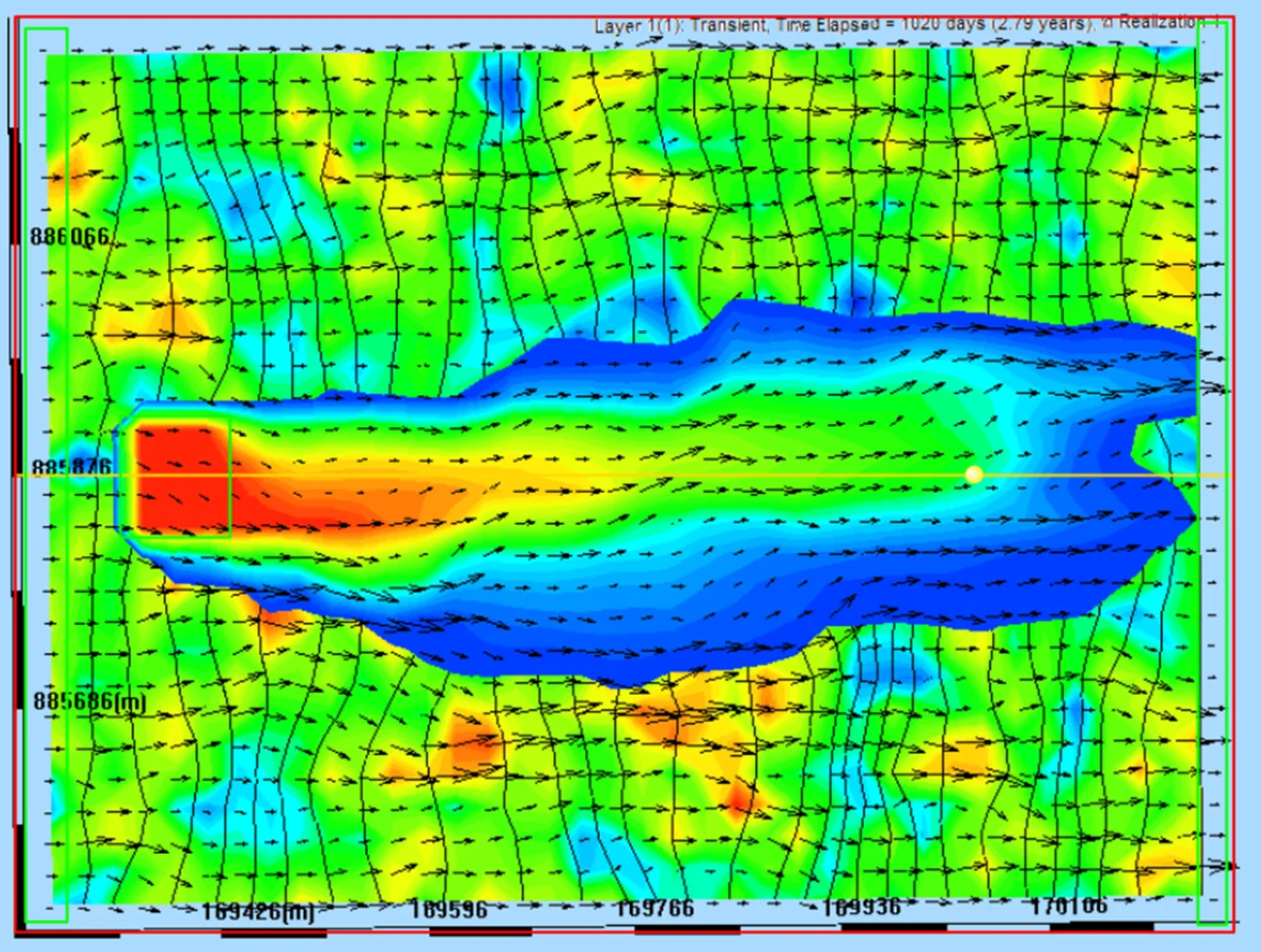
Compare the single-realization result against a uniform-K baseline run of the same model. You'll see, qualitatively:
- Head contours irregular — they distort around low-K bodies where flow is impeded and concentrate in high-K channels where flow runs freely
- Flow vectors bend and channel — rather than following smooth parallel paths from source to sink, vectors deflect around low-K zones and concentrate in high-K pathways, producing spatially-variable magnitudes
- Particle paths tortuous — paths twist as they navigate the random structure, with some particles moving quickly through high-K corridors and others taking meandering slow routes
- Travel times spread — particles that started together arrive at outlets at very different times, reflecting the diversity of path conductivity experienced
19.4.2 What a single realization is and is not
Critical framing:
- Is: one physically-plausible arrangement of the aquifer consistent with the specified statistics
- Is: a visualization of heterogeneity effects that uniform-K modeling cannot show
- Is: a useful hypothesis for planning, design, or exploratory analysis
- Is NOT: "the truth" about the actual aquifer in the ground
- Is NOT: a prediction with quantified uncertainty — without an ensemble, you don't know how this specific realization compares to other possible realizations
- Is NOT: sufficient for regulatory or risk-based decisions that require uncertainty bounds
19.4.3 When single-realization work is enough
Single realization suffices when the question is:
- "What does flow through a realistic heterogeneous aquifer look like?" (teaching, client communication)
- "Can low-K zones plausibly deflect a contaminant plume in unexpected directions?" (exploratory)
- "Does the heterogeneity structure produce preferential flow that could route contamination to a specific well?" (screening)
- "Is the flow field qualitatively sensitive to heterogeneity?" (testing whether ensemble analysis is warranted)
Escalate to ensemble when the question requires probability or risk language — confidence intervals, exceedance probabilities, percentile bounds, risk-weighted decisions. Those require the ensemble (§19.5).
19.5 Ensemble Monte Carlo Simulation
Ensemble Monte Carlo runs many realizations — tens to thousands — and aggregates them into ensemble statistics. This is where uncertainty quantification happens. The setup extends the single-realization setup with a realization count and ensemble output options.
19.5.1 The Monte Carlo setup workflow
Configure the random field(s)
Identical to single-realization setup: zone-level isRandom flags, correlation scales, variance, mean. Each realization will use these statistics but a different random seed.
Enable Monte Carlo in Solver Options
Check Monte Carlo Simulation in the Solver Options dialog. Specify the number of realizations. Start with 10-20 to verify the setup works; scale up to 100-1000 or more for production uncertainty quantification.
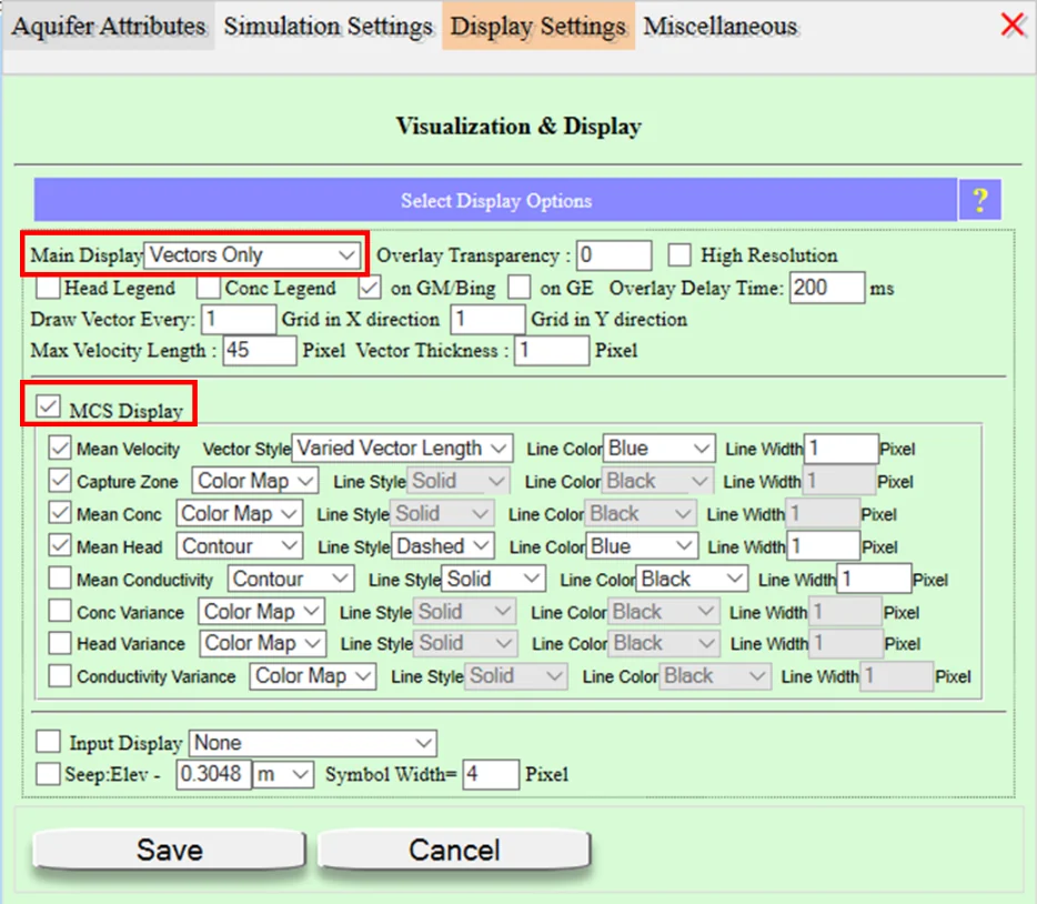
Configure MCS Display options
In the MCS Display section, check what you want to visualize as the ensemble accumulates: Mean Head, Head Variance, individual realizations (to watch the ensemble form), mean flow vectors, current-realization flow vectors. Typical choice for flow: check Mean Head and Head Variance, so you see the ensemble mean smoothing and the variance map building up.
Add Monitoring Probability at critical points
Place monitoring wells at points where you specifically need probability distributions (e.g., a public-supply well for which you want a contaminant risk assessment). Check the Monitoring Probability checkbox on each well. IGW-NET will record the head (and concentration, if transport is active) value at this location for every realization, building up a probability distribution.
Launch and watch
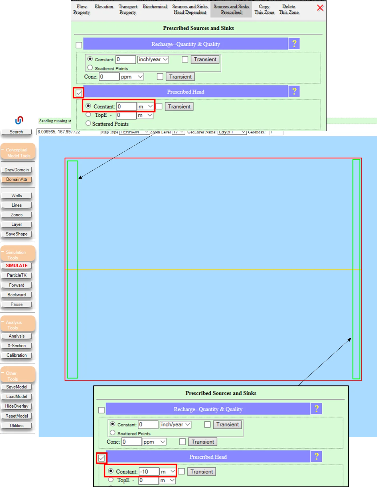
Simulation proceeds realization by realization. Each realization's flow (and transport) is computed; ensemble statistics update; you see the mean fields smoothing, the variance maps filling in, the monitoring-well probability distributions populating. You can stop when the statistics have visibly converged — no need to predetermine the exact realization count.
19.5.2 Watching the ensemble form
19.5.3 How many realizations
Common question without a rigid answer. Guidelines:
- For mean fields (ensemble mean head, ensemble mean concentration): 50-100 realizations often converge adequately. Watch the mean field visualization; when it stops changing noticeably as new realizations add, you've converged.
- For variance fields (head variance map): 100-500 realizations typical. Variance converges more slowly than mean.
- For probability tails (exceedance probabilities, 5th/95th percentile): 500-1000+ realizations. The rarer the event you're trying to quantify, the more realizations you need to see it reliably.
- For probabilistic capture zones: 100-500 is typical; the fuzzy boundary structure stabilizes at this range.
Because IGW-NET's recursive-statistics architecture (§19.6) has no memory penalty for larger realization counts, there's no strong reason to under-run. When in doubt, run more. Watch convergence in the real-time visualization and stop when statistics stabilize.
19.6 The Recursive-Statistics Architecture — Why This Works at Scale
Ensemble Monte Carlo at fine grid resolution is traditionally prohibitive because storing the ensemble is prohibitive. IGW-NET's recursive-statistics architecture eliminates that constraint. This section explains the mechanism and why it matters.
19.6.1 The storage problem
Consider a realistic 3D groundwater model: 10⁶ cells (say 1000 × 1000 × 1 layer for a 2D model, or 200 × 200 × 25 layers for 3D). You run 1000 realizations of Monte Carlo simulation. The naive approach stores every realization's head field, then post-processes the ensemble to compute statistics:
- Storage per realization per variable: 10⁶ × 8 bytes = 8 MB
- Storage for 1000 realizations of heads alone: 8 GB
- Plus concentrations, fluxes, other outputs: quickly into tens of gigabytes
- Post-processing to compute statistics: read the whole ensemble back; compute mean, variance, percentiles; write statistics maps
At these sizes, the workflow starts choking. Disk I/O becomes the bottleneck. Memory pressure causes swapping. The user can no longer interactively explore the results — they're locked into a batch-processing pattern. And it only gets worse with finer grids (the grid cell count scales with the cube of linear resolution in 3D) or more realizations.
19.6.2 The recursive solution
IGW-NET never stores the ensemble. Instead, each realization updates running statistics in place, then is discarded. The running statistics have the same memory footprint as a single realization's output, regardless of how many realizations have been processed.
For the ensemble mean at cell (i,j,k) after N realizations:
mu_N = mu_{N-1} + (h_N − mu_{N-1}) / N
Each realization's head h_N is incorporated into the running mean mu and then discarded — no need to ever store h_N again.
For the ensemble variance, IGW-NET uses Welford's online algorithm, which computes running variance numerically stably without accumulating round-off errors (naive cumulative-sum-of-squares algorithms become unstable for large N):
M2_N = M2_{N-1} + (h_N − mu_{N-1}) × (h_N − mu_N)
variance_N = M2_N / N (or M2_N / (N−1) for sample variance)
Probability-of-exceedance fields work similarly: maintain a count of realizations exceeding a specified threshold at each cell, divided by N, updated per realization. Percentiles require slightly more work but are also computable via online algorithms or streaming quantile estimators.
Each realization: compute the flow solution, render the current-realization visualization, update running ensemble statistics, update ensemble-mean and variance visualizations, discard the realization-specific data. Start the next realization.
Memory cost: O(cells × number of statistics types). Not O(cells × realizations).
This is the same pattern IGW-NET uses for transient simulation — each time step is computed, displayed, incorporated into time-series statistics, and discarded. Transient simulations aren't limited by the number of time steps you can visualize; they're limited only by compute time. The stochastic architecture reuses the pattern: Monte Carlo simulations aren't limited by the number of realizations you can visualize; they're limited only by compute time.
19.6.3 What you can do because of this
Practical consequences of the recursive-statistics architecture:
- Run as many realizations as you want. 10, 100, 1000, 10,000 — the memory footprint is the same. Run whatever you need for statistical convergence; stop when visualizations stabilize.
- High-resolution 3D ensembles are tractable. Where traditional tools force you to coarsen the grid to fit the ensemble in memory, IGW-NET runs at full model resolution regardless of realization count.
- Real-time convergence monitoring. Watch the mean field smooth and the variance map stabilize as realizations accumulate. Decide when to stop based on what you see, not on a pre-specified count that might be too small or too big.
- Iterative exploration. Try a setup with 20 realizations for quick feedback; if you like what you see, continue with 200 more to refine statistics. The workflow is responsive at every step.
- Consistent with interactive modeling philosophy. IGW-NET's whole design philosophy (Ch. 18 §18.1.3) is about making model iteration fast and interactive. Stochastic analysis fits into this philosophy rather than forcing a batch-processing exception.
19.6.4 What trades off
The recursive approach has minor limitations worth noting:
- Specific percentile information is limited. Running statistics give mean, variance, and probability-of-exceedance at pre-specified thresholds naturally. Arbitrary percentiles (e.g. "what's the 27th percentile at this cell?") require either storing more information or accepting approximations.
- Retroactive analysis is limited. Once the ensemble is done, you cannot go back and ask "what do the realizations with low K look like in aggregate?" — those realizations aren't stored. For questions like this, selectively record subsets of realizations at specific points of interest (IGW-NET's Monitoring Probability checkbox does this for wells) or save a smaller ensemble sample.
- Debugging a specific unusual realization is harder since you can't revisit it. Use a deterministic seed for reproducibility if you want to re-run a specific case.
In practice these trade-offs are small compared to the massive gain in ensemble capacity.
19.7 Result Interpretation — From Ensemble to Insight
Running the ensemble is the mechanical step. Interpreting the ensemble statistics is where the value is extracted. This section covers the main output types and their interpretation.
19.7.1 Mean head field
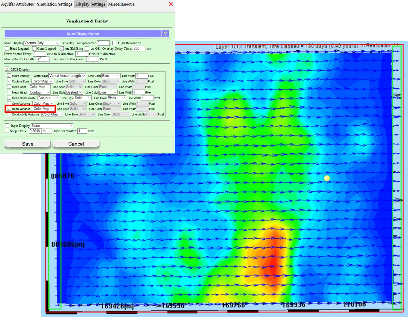
The ensemble mean head at each cell is the expected head value averaging over the uncertainty in K. It's smoother than any single realization because the ensemble averages out realization-specific heterogeneity patterns. For most purposes (regional water budget, typical head pattern, average flux estimates), the mean is what you want.
19.7.2 Head variance map
Typical interpretation patterns:
- Low variance near boundaries: BCs pin the head regardless of K, so variance is minimal
- Higher variance in the interior: K has more room to affect heads when no BC is nearby
- Peaks near pumping: drawdown depends sensitively on local K, so regions near heavy pumping often have high variance
- Peaks at SW-GW boundaries: leakance and K both affect exchange, compounding uncertainty
19.7.3 Probability distributions at monitoring wells
Where Monitoring Probability was enabled, IGW-NET records head (and concentration, if active) values from every realization at that specific well, producing a probability distribution. The chart shows a histogram or density curve — "at this well, the head is most likely between X and Y, with some probability of being lower or higher."
Typical uses:
- "What's the probability that head at this well exceeds a specific threshold?" — read off the exceedance probability from the cumulative distribution
- "What's the 5th–95th percentile range for head at this well?" — confidence interval for engineering design
- "Is the well likely to go dry under a specified scenario?" — compute P(head below well bottom) from the distribution
19.7.4 Macrodispersion in transport ensembles
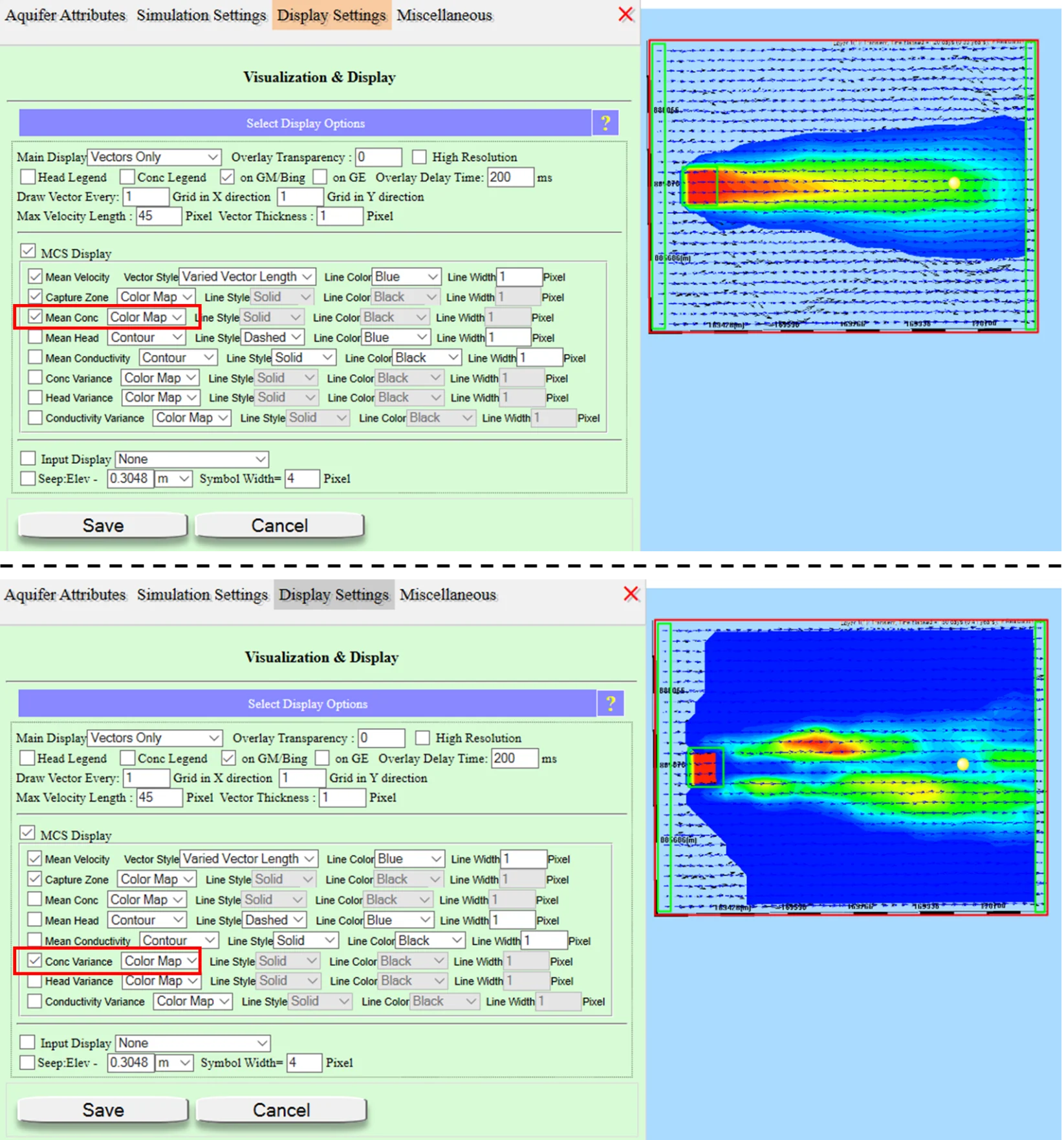
Macrodispersion is the excess spreading of the ensemble mean plume beyond any single realization's plume. Different realizations route contaminants along different preferential pathways; averaging them produces a smoother, wider mean plume. Macrodispersion is a fundamental property of heterogeneous aquifers — it cannot be captured by a uniform-K model with a tuned dispersivity parameter; it's a real physical phenomenon emerging from K heterogeneity.
Concentration variance at the plume fringe is diagnostic of contamination risk. Low variance in the plume interior (always contaminated); low variance far ahead of the plume (always clean); high variance in the transition zone (maybe contaminated, maybe not). The variance map highlights locations where small K-field differences produce large concentration differences — where the contamination risk is genuinely uncertain.
19.7.5 Probabilistic capture zones
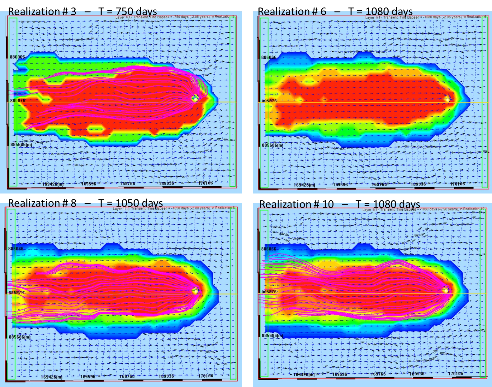
A probabilistic capture zone replaces the deterministic "this polygon is inside the capture zone" with "each location has probability P of being captured." Useful applications:
- Wellhead protection area designation: protect all locations with capture probability above a chosen threshold (e.g., 10% for conservative, 50% for less conservative)
- Contaminant source tracking: given contamination at a specific well, what's the probability each potential source reached it?
- Source-control prioritization: among known contamination sources, rank by capture probability for the affected well — highest probability = most likely contributor
19.8 Connection to Calibration — Parameter Uncertainty as Stochastic Input
Stochastic modeling and calibration (Ch. 18) naturally connect. UCODE parameter estimation produces not just optimal parameter values but parameter uncertainty — standard errors, correlation matrices, confidence intervals on parameters. Those uncertainty estimates are directly usable as inputs to stochastic analysis.
19.8.1 UCODE output as stochastic input
After running Automatic Calibration with UCODE (Ch. 18 §18.7), you have:
- Optimized parameter values (e.g., K multiplier = 0.3)
- Parameter standard errors (e.g., K multiplier = 0.3 ± 0.05)
- Parameter correlation matrix (e.g., K multiplier and Recharge multiplier correlated at 0.8)
These together define a multivariate distribution of plausible parameter values consistent with the calibration data. You can use this distribution to drive stochastic analysis:
- Sample parameter values from the UCODE-derived distributions (accounting for correlations)
- For each sampled parameter set, run the model
- Aggregate outputs across samples into ensemble statistics
The result is uncertainty quantification that propagates calibration uncertainty into simulation outputs. A prediction (say, head at a new well site) now has a confidence interval derived from the calibration's own uncertainty — not an arbitrary guess.
19.8.2 Combined parameter and heterogeneity uncertainty
Advanced stochastic analyses combine multiple uncertainty sources:
- Parameter uncertainty (from UCODE): uncertainty in calibrated multipliers
- Heterogeneity uncertainty (from SGS/T-PROGS): uncertainty in the spatial K distribution
- Boundary condition uncertainty (where applicable): uncertainty in prescribed heads or fluxes
Each realization draws from all three sources jointly: one K multiplier sampled from UCODE distribution, one SGS K field generated with a different random seed, one BC value sampled if that's in play. The resulting ensemble captures all three sources of uncertainty together.
IGW-NET supports this compound stochastic analysis natively — the isRandom flags work at multiple levels (multiplier-level for UCODE-derived parameter uncertainty; zone-level for heterogeneity; boundary-level for BC uncertainty). The recursive-statistics architecture works identically regardless of how many uncertainty sources are active.
19.8.3 Parameter uncertainty vs. structural uncertainty
An important limitation. Ensemble Monte Carlo, whether driven by UCODE parameter uncertainty, SGS heterogeneity, or both, quantifies uncertainty within a fixed model structure. It does not quantify whether the structure itself is correct. If your layering, BCs, or fundamental conceptual model is wrong, Monte Carlo will give you a very confident confidence interval on the wrong answer.
This connects to Ch. 18 §18.1.3 — structure first, calibration and stochastic analysis second. Stochastic modeling refines the understanding of a structurally-sound model; it cannot rescue a structurally flawed one. The narrow confidence intervals of a Monte Carlo ensemble on a wrong structure are more dangerous than wide confidence intervals on a sound one — the tight statistics give false confidence in predictions that may still be very far off.
Before stochastic analysis, use IGW-NET's real-time modeling and visualization to verify the structure is defensible. Stochastic analysis then quantifies the residual parameter and heterogeneity uncertainty within that sound structure.
19.9 Common Pitfalls
Stochastic modeling has its own failure modes, distinct from deterministic modeling pitfalls. This section collects the common ones.
19.9.1 Single realization mistaken for the answer
A single realization is one hypothesis — one possible arrangement consistent with the statistics, not "the truth." Users who generate a single realization and interpret its specific patterns as real are over-reading. The patterns in one realization reflect that specific random seed; a different seed would produce different patterns.
Fix: either frame the single realization explicitly as "one plausible hypothesis" for exploratory or communication purposes, or escalate to ensemble analysis. Don't report single-realization results as "the stochastic answer."
19.9.2 Correlation scale misconfiguration
Setting LambdaX too small produces near-independent noise; too large produces near-constant fields. Both break the realism of the random field. Users who leave defaults without thinking about the geological setting often get unrealistic heterogeneity patterns.
Fix: match LambdaX, Y, Z to the geological feature lengths. Horizontal 100-2000 m for most sedimentary aquifers; vertical 1-10 m reflecting layer thicknesses. §19.3.3's tip callout covers this.
19.9.3 Too few realizations
Running 10 realizations and declaring the statistics converged is almost always wrong. Mean fields need dozens; variance maps hundreds; probability tails thousands. Premature stopping produces ensemble statistics that reflect the specific realizations chosen more than the underlying distribution.
Fix: watch convergence in IGW-NET's real-time visualization (§19.6 enables this). Continue until statistics visibly stop changing. With the recursive-statistics architecture, running more realizations has no memory penalty.
19.9.4 Treating realizations as independent when they shouldn't be
If parameter uncertainty and heterogeneity uncertainty are both active, sampling them independently may miss important correlations. For example, if UCODE finds K and Recharge strongly correlated (the non-uniqueness from Ch. 18 §18.8), sampling them independently produces (K, R) pairs that contradict the calibration. Honoring the correlation structure matters.
Fix: sample multi-variable parameter distributions with their covariance structure, not as independent univariate distributions. UCODE-derived distributions have correlation matrices — use them.
19.9.5 Structural uncertainty ignored
Covered in §19.8.3 and in the key callout. Monte Carlo quantifies parameter uncertainty within a fixed structure; structural uncertainty is bigger and not captured. Modelers who report tight confidence intervals from a Monte Carlo ensemble without acknowledging that the structure could be wrong are overselling.
Fix: always frame Monte Carlo results as "parameter uncertainty within this structure" and separately address structural uncertainty through sensitivity analyses (try alternative structures, compare results) or through explicit discussion of the structural assumptions.
19.9.6 Realistic appearance without observational backing
SGS produces visually impressive K fields that look realistic even when the specified statistics aren't based on anything real. Users who set variance, correlation, and mean to plausible-looking numbers without empirical justification get plausible-looking results that may have no defensible statistical basis.
Fix: ground the random field parameters in data where possible — borehole spacing analysis for correlation scales, pump test variability for K variance, published regional studies for typical values. When data is limited, explicitly acknowledge the parameters are assumptions.
19.9.7 Using ensemble mean as "the answer"
The ensemble mean is one useful statistic but not "the answer." Planning decisions based on the mean alone ignore the spread — decisions robust to the mean may fail under realistic realizations. Conversely, worst-case planning based on the tail alone ignores typicality — overly conservative decisions waste resources.
Fix: use the full statistical output. Plan for the mean behavior; stress-test against percentile bounds; make decisions explicitly risk-informed by the probability structure. The whole point of the ensemble is to enable this richer decision-making.
To go deeper
- Chapter 17 — T-PROGS 3D Geology — the categorical-variable counterpart to SGS; the other half of IGW-NET's spatially-correlated-random-field toolkit.
- Chapter 18 §18.7 — Automatic Calibration with UCODE — parameter uncertainty output that feeds stochastic input; Section 18.1.3 on structure-first.
- Chapter 11 §11.4 — Backward particle tracking — the method behind probabilistic capture zones.
- Chapter 12 §12.6 — Dispersivity — local dispersion parameters that combine with macrodispersion from stochastic heterogeneity.
- Chapter 20 — MODFLOW Integration → — next chapter. Exporting calibrated and/or stochastic IGW-NET models to MODFLOW for external workflows.
- Realtime help: Random Field Options — operational reference for the random field dialog.
- Realtime help: Random Field Parameters — parameter-by-parameter reference.
- Tutorial 15: Stochastic Flow — single-realization walkthrough.
- Tutorial 16: Monte Carlo Flow — ensemble Monte Carlo walkthrough.