To add a surface water body that has significant areal extent, that is, it cannot be approximated using a single line, it is necessary to define the location and geometry of this surface-water body. To do this click on Conceptual Model Tools and then on Zones. Several options will be available (see Figure 37).
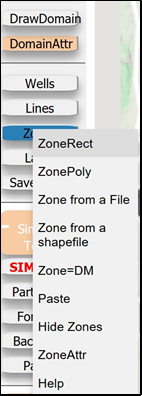
Figure 37: Window used to select zone.
Now click on ZonePoly. This will provide you with a plus sign as a cursor with which you can draw a polygon. To draw the polygon, click on a point on the model that is on the border of the area you wish to designate as the surface water body. Next move a small distance along the perimeter of the surface water body and click again. You have now created a polygon with two points. Not very interesting! Continue to move around the surface water body in small increments, clicking at the end of each increment, until you return to the location at which you started. Click once again on the first point you generated. You have now completed the polygon. An example is shown in Figure 38. The area within the polygon is your lake.
To give the lake descriptive physical parameters, click ‘SaveShape’; alternatively, you can do the following. Return to Conceptual Model, click Zone, and then click on Zone Attr to access the parameter input page. The drop down menu (Figure 39) reveals that we have only one zone, so we click on that. This spawns the following message (Figure 40) to which we respond OK. Along the top of the window there are several options. This is because this ribbon is used to provide input for six different situations. Each choice can be used to define properties within your polygon. So, for example, if you wanted to define a different hydraulic conductivity over a specific region of the model than what occurs elsewhere in the model, you could draw a polygon to define the area where you want the different hydraulic conductivity and then enter the value for that region. It will replace the one originally assigned in that region with your value.
However, we digress, we are actually interested in the properties of the lake we have defined. To make changes to the lake we click Sources and Sinks Head Dependent (Figure 41). In the upper left-hand corner of this figure we see the notation Two-way Head Dependent. This is the panel we need, but what it means requires a little explanation.
We need to be able to have water either enter or leave the lake depending upon the relative elevation of the hydraulic head below the lake (in our model) and the elevation of the lake surface. For example, if there is a period of drought when the lake level is low so there is a hydraulic head in the aquifer below the lake that is higher than the water level in the lake, we need to have water move from the groundwater system to the lake. In other words, at the interface between the stream bottom and the aquifer there would be a negative gradient from the aquifer to the lake. On the other hand, if there is abundant rainfall and the river level is higher than that in the aquifer, we would expect water to flow from the river into the aquifer. This situation where water can either enter or leave is defined as a ‘Two-way Head Dependent’ condition because water can either enter or leave the lake depending upon hydrologic circumstances.
Returning to the upper left-hand window we see that we have a Lake defined (see window adjacent to Name). The stage is the elevation of the water level in the lake relative to a reference elevation. It can be specified as a number that is constant in time and space. If this is your choice you click the radio button next to Const and specify a value.
It is often convenient to check the option TopE for the stage where TopE is the top elevation taken from the map (DEM). If you wanted to modify the choice from the DEM, you can replace the value in the box adjacent to the TopE notation with a suitable value. For example if you wanted to have the stage one meter lower than the elevation determined from the DEM, you would replace the zero with a one. Once the table is filled in, click the little white box to the left of the heading ‘Two-way Head’ and then click SAVE.
One sees that there are two other options for how one treats the lake. These choices are variants on the one we have selected and their specific attributes can be determined by clicking the ? at the end of each descriptive title.
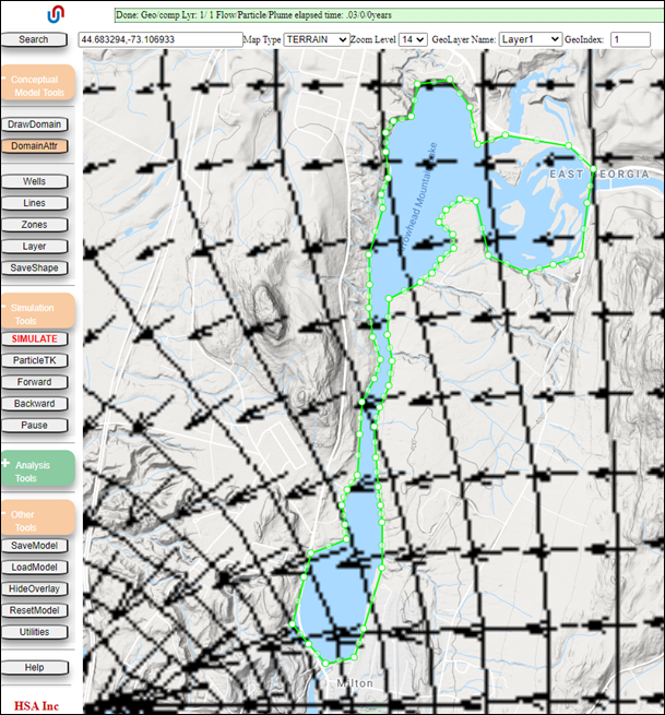
Figure 38: Polygon representation of a lake near Milton, Vermont.
.
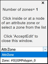
Figure 39: Selecting a zone for editing.
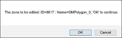
Figure 40: Prompt indicating the polygon feature to be edited if you proceed by clicking ‘OK’.
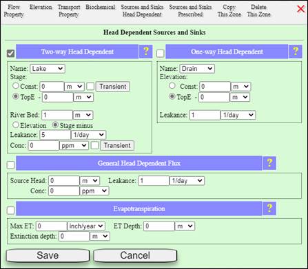
Figure 41: Option selection for flow from or to a lake.
The next step is to simulate the behavior of our aquifer with the lake included. This is achieved by clicking the SIMULATE button, whereupon the sequence of messages shown in Figure 42 and Figure 43 are encountered. Check OK for each and your simulation will begin. Note that the progress of the simulation appears at the top of the screen in the message window. In due course the computed head solution for the entire model is produced and plotted. The specific area of interest to us is shown as Figure 44.
The specifications provided effectively make the lake a local groundwater source, that is to say that water flow is out the lake into the aquifer. Flow from the lake to the aquifer would occur if, for example, there was a significant rainfall event that raised the water level in the lake relative to the hydraulic head in the aquifer under and around the lake. Note that the contours to the right (east) are higher than those to the left (west) in both figures. However, if you can imagine being in the center of the lake, you would be on a hydraulic head ‘hill’ with the hydraulic head surface sloping down to the north and also down to the south. This observation supports the fact that water is moving from the lake into the aquifer. Had the lake been receiving groundwater from the aquifer the ‘hill’ would be replaced by a ‘depression’.
Note that a new cross-section (yellow line segments) was drawn in the submodel domain as shown in Figure 44. As described in Section 4.2, to draw a new cross-section at any time, go to Analysis Tools and then click X-Section. After you have finished drawing the cross-section, go to Analysis Tools and click the Analysis button. From the list of options, click Display Charts. The new cross-section results will be shown in the Cross Section Diagram and Cross Section Plot charts (see Figure 45). Also note the updated water balance (amount of water moving into and out of the system) now includes Lake terms to represent flow to or from the lake (negative flux = groundwater lost to the lake; positive flux = lake water added to the aquifer).
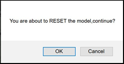
Figure 42: Warning message in preparation for simulation.
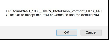
Figure 43: Second warning message prior to simulation.
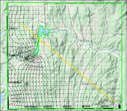
Figure 44: Calculated hydraulic head surface when groundwater is being recharged by the lake.
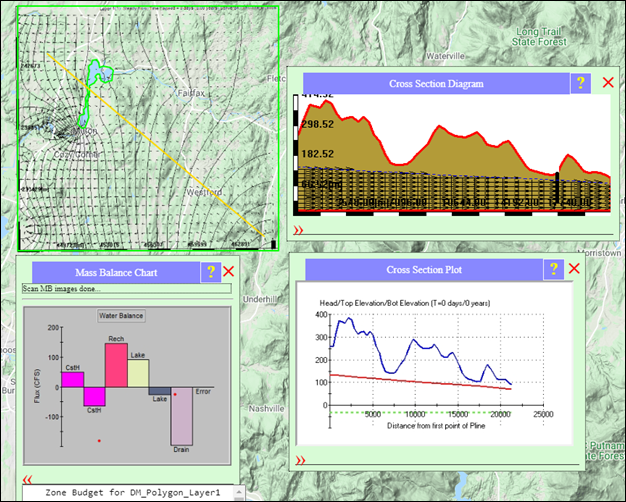
Figure 45: Submodel results, including plan view flow field and velocities; cross-section diagrams/plots, and an updated water balance chart.