Next, we want to delete the information provided for the particles calculations because we are going to model transport which is dependent not only on groundwater convection (represented by particle paths), but also on diffusion and dispersion and this involves a new approach. To apply this new approach , click on Simulation Tools, then click Particles, then click DeleteParticle. This removes any particle features included in the model domain, including the particle rectangle. Note that the pathlines will not be removed until a new simulation is returned to the map display.
We will want to visualize the computed plume in both plan view and cross-sectional view when we re-submit our data set for simulation. First use the X-section tool under Analysis Tools to draw a new cross-section through the center of the “potential impact area” determined from particle tracking (see Figure 67).
Now we are ready to submit the model for flow and transport simulation (click SIMULATE). Again, the flow field is steady (does not change with time), but the contamination plume will evolve over the course of the simulation and the results are shown in the map display (Figure 68). We can see significant spreading of the plume, caused by applying longitudinal dispersion and by the relatively coarse grid size (NX=40). The coarse grid size causes “numerical dispersion” or artificial spreading due to numerical approximation error when numerically solving the transport equations.
The cross-section diagram (accessed under Analysis Tools, Analysis, then Display Charts) shows a plume that is vertically-mixed, which is consistent with the fact that we are simulating two dimensional groundwater flow in this example (i.e., no resolution of vertical details). In the next section, we will learn how to resolve vertical details by adding more layers to the model.
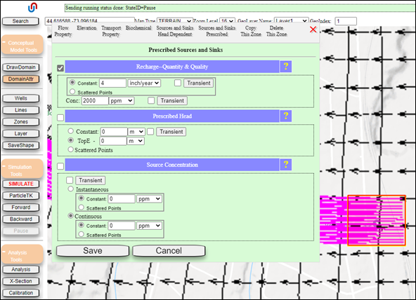
Figure 66: Source of dissolved species assigned in the Prescribed Sources and Sinks tab of the Zone Attributes menu.
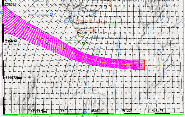
Figure 67: Cross-section drawn through the center of the probable impact zone as predicted by the forward tracking analysis.
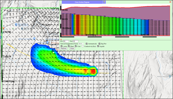
Figure 68: Snapshot of simulated transport results (plan view and cross section view).