Now, to access the multiple layers option (that is, the ability to define the number of computational layers for a given geological layer), click on the Simulation Tools tab at the top of the Domain Attributes menu. This then reveals the Simulation Settings window shown in Figure 69. Now click the box to the left of Number of SubLayers and put in the box to the right of Number of Sublayers the number of layers you require.
You should also check the box next to ‘Water Table as Top’. This tells MAGNET to subdivide the aquifer following the simulated water table of your last model submitted to the MAGNET server (you can also upload a saved model result). It is good practice to first simulate the two dimensional water table, then add computational layers and sub-divide following the two dimensional water table.
Click SIMULATE to solve the new model with multiple computational layers. When you view the results in the cross-section diagram, you will see that the chemical source is being now added to the top of the aquifer or the 1st computational layer (see Figure 70). You will also see the different computational layers as yellow dotted lines.
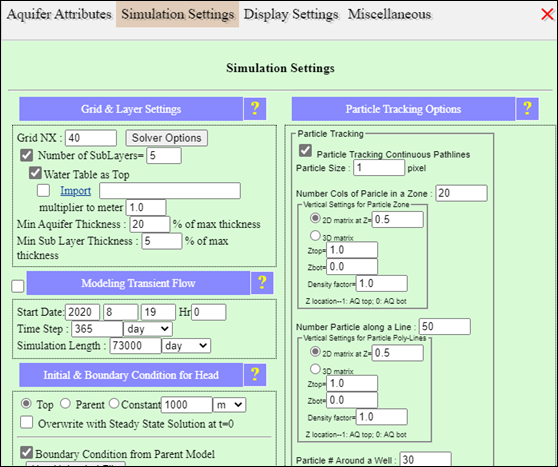
Figure 69: Window used to add computational layers to the model.
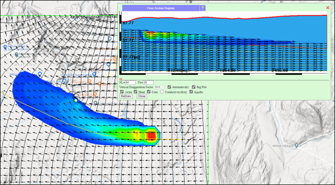
Figure 70: Simulated flow field and contaminant transport with five computational layers.