Define the watershed region on the map.
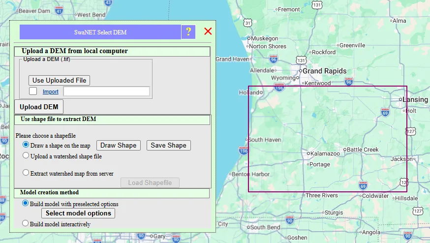
Login to SwaNET. Zoom into the region of interest. Create a new project, draw a box on the map covering the watershed, and save the shape.
SwaNET does the heavy lifting — terrain, soil, land use, climate, stream networks, HRUs, simulation, visualization, monitoring data — so a working watershed model arrives in minutes. The model is the starting point. You spend your time on what changes the answer: refinement, comparison, calibration, scenarios.
Conventional watershed modeling spends weeks on data assembly before the first simulation. SwaNET inverts this. Pre-processed multi-resolution data is already on the network. Watershed and subbasin delineation, stream networks, land use and soil extraction, HRU computation, weather generation, SWAT input writing, and the simulation itself — all are automated inside the platform.
The first model is reasonable, detailed, and ready to interpret in a few minutes. It is not the final model. It is the starting point that frees you to do the work that actually changes the answer: experimentation, scenario testing, model-data comparison, management interpretation.
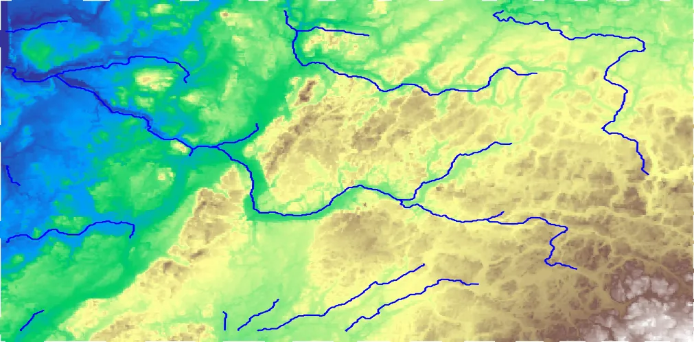
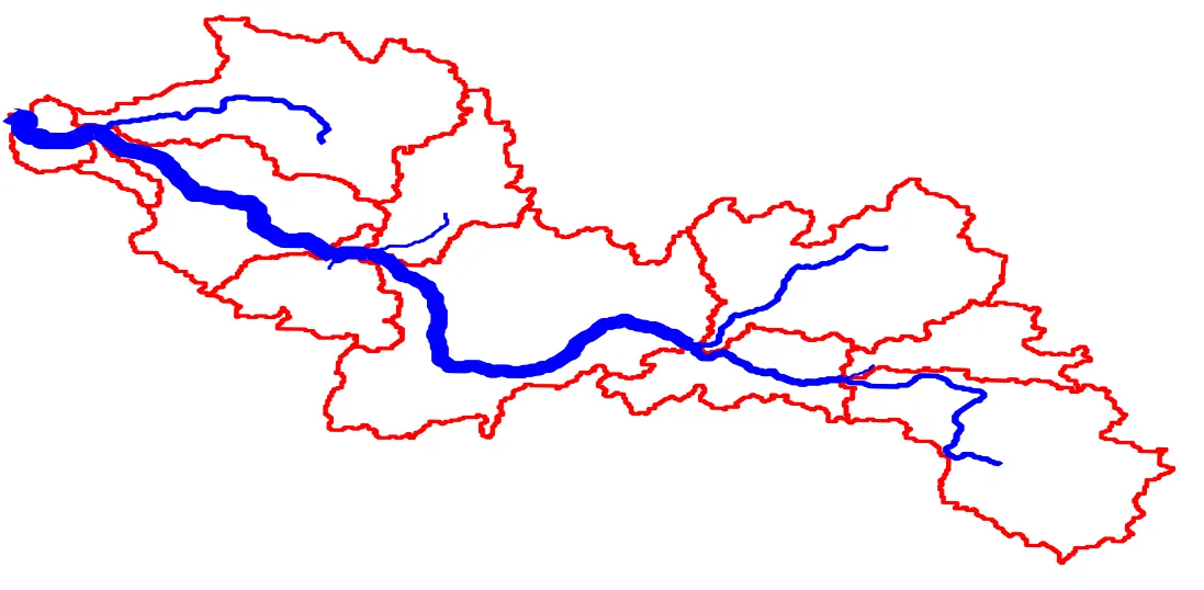
Terrain + streams
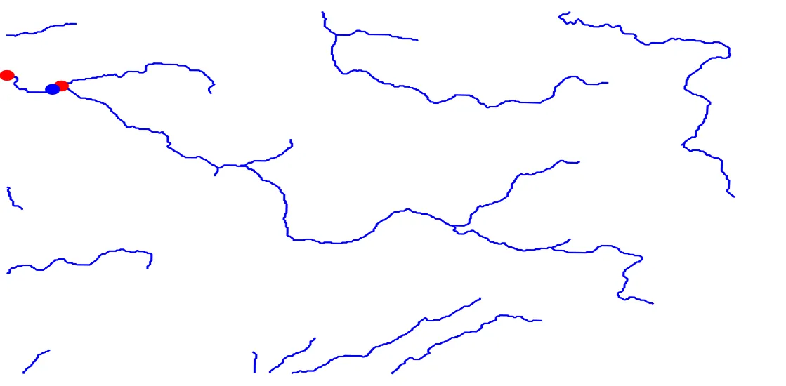
Snapped outlet
Watershed + subbasins
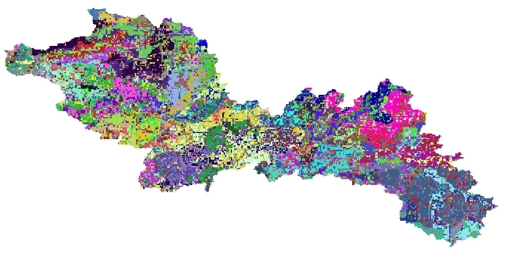
Land use
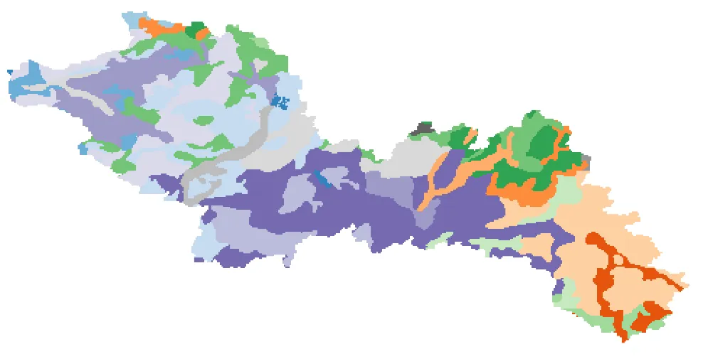
Soil type
Signature
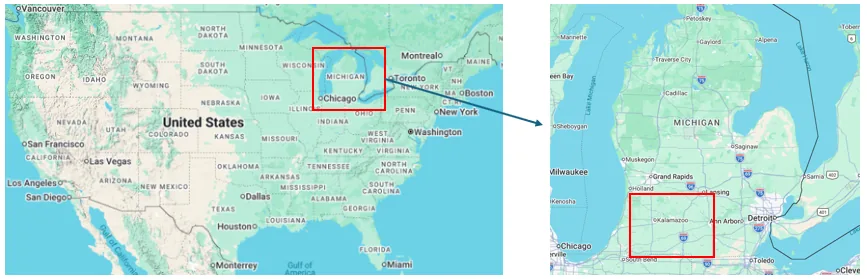
Four steps from login to a working watershed model. The example is the Kalamazoo River Watershed in southwestern Michigan, but the workflow is the same for watersheds across the United States, Canada, and most regions worldwide where the underlying data services are available.
Login to SwaNET. Zoom into the region of interest. Create a new project, draw a box on the map covering the watershed, and save the shape.
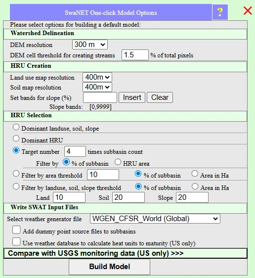
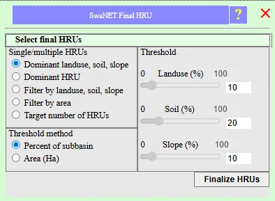
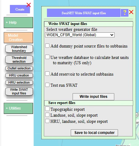
For the first model, accept every default. Defaults are calibrated starting values — well-chosen, sensible, and fast.
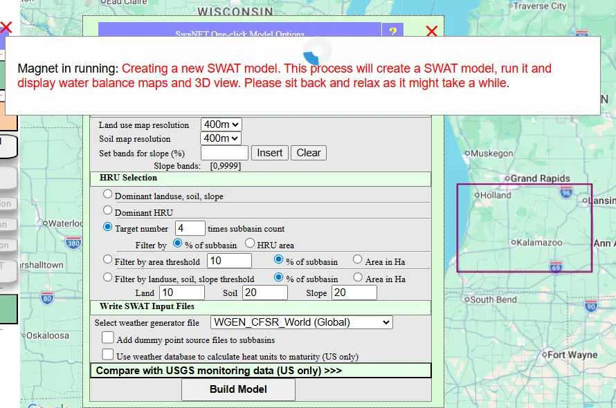
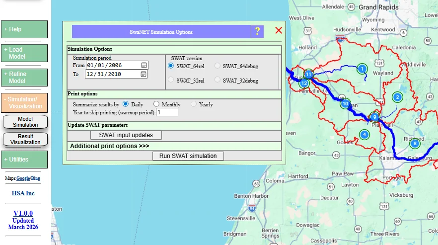
Wait a few minutes. During this time, pre-processed big data for the model area is extracted, all model input files are created, and the simulation runs — model building and visualization happen automatically.
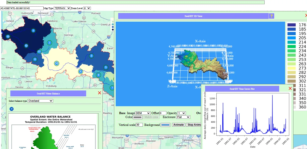
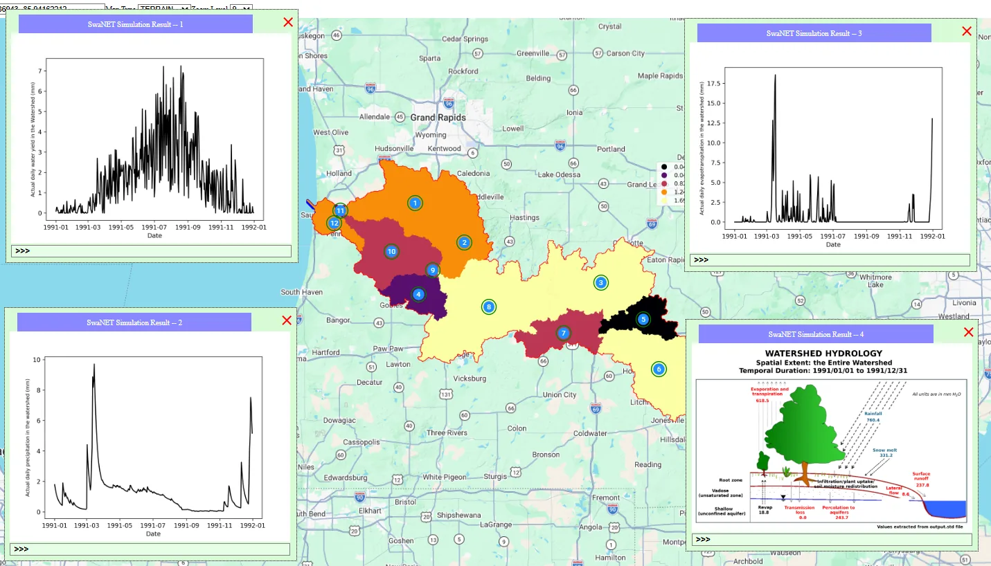
Once the simulation finishes, results appear automatically in the map display and pop-up interfaces. Three views show themselves first — each answers a different question.
1990–1991 with 1990 as spin-up year if not.
SwaNET's auto-displayed outputs aren't a generic dashboard — each view is a different lens on the same simulation, designed to answer a different question. Read them in this order.
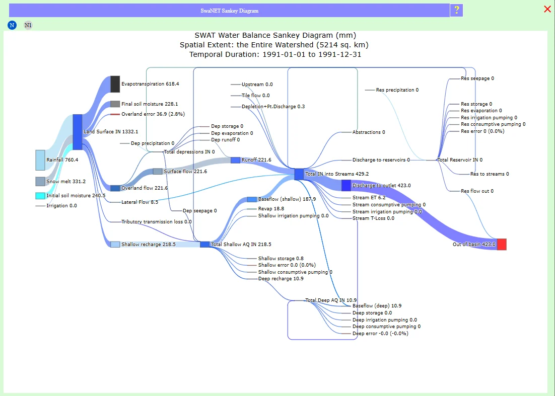
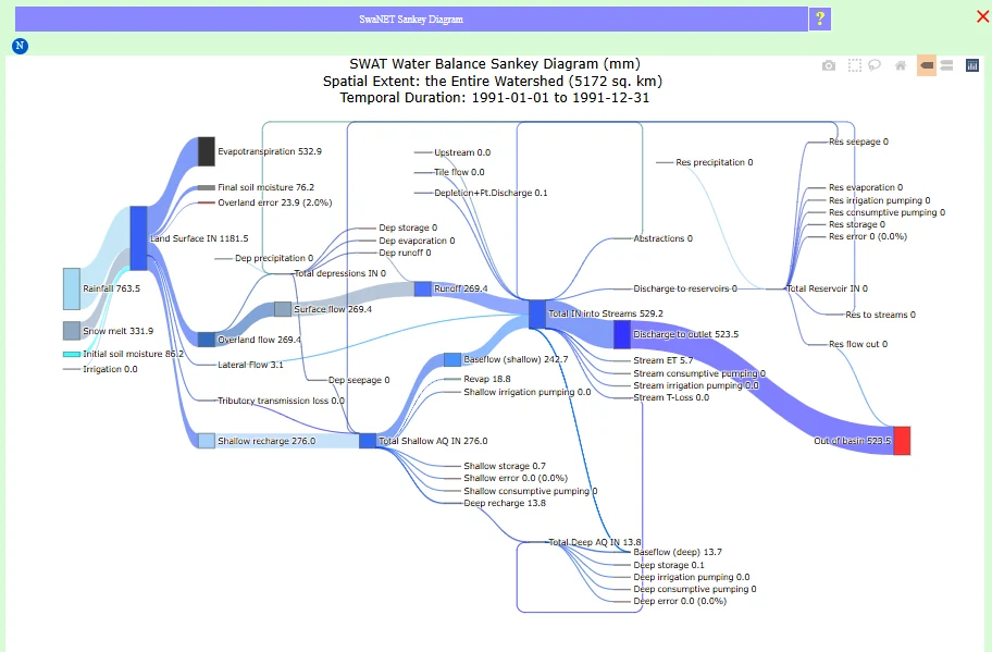
Sankey · System water balance
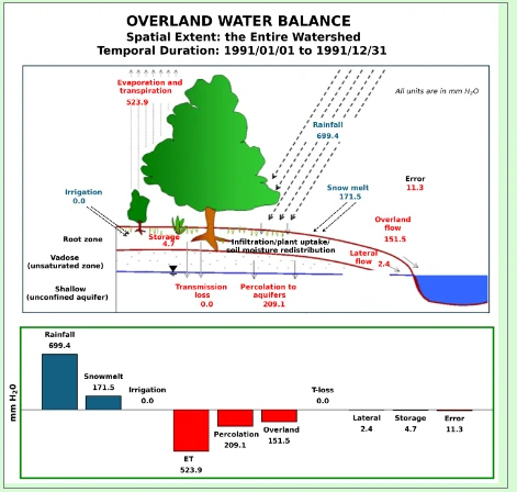
A complete, quantitative description of all inflows, outflows, and stocks in the watershed — and how they connect. The watershed's hydrologic fingerprint in one image. If the simulation spans multiple years, multiple Sankey diagrams are produced.
Streamflow time-series
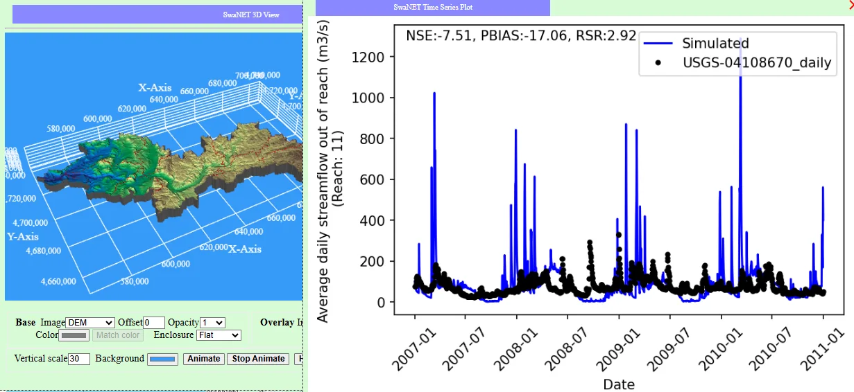
Streamflow at the watershed outlet over the simulation period. Reveals the regime — base-flow dominance, flashy response, seasonal pattern, peak timing. This is where observed data will overlay once you load gauge stations.
3D watershed visualization
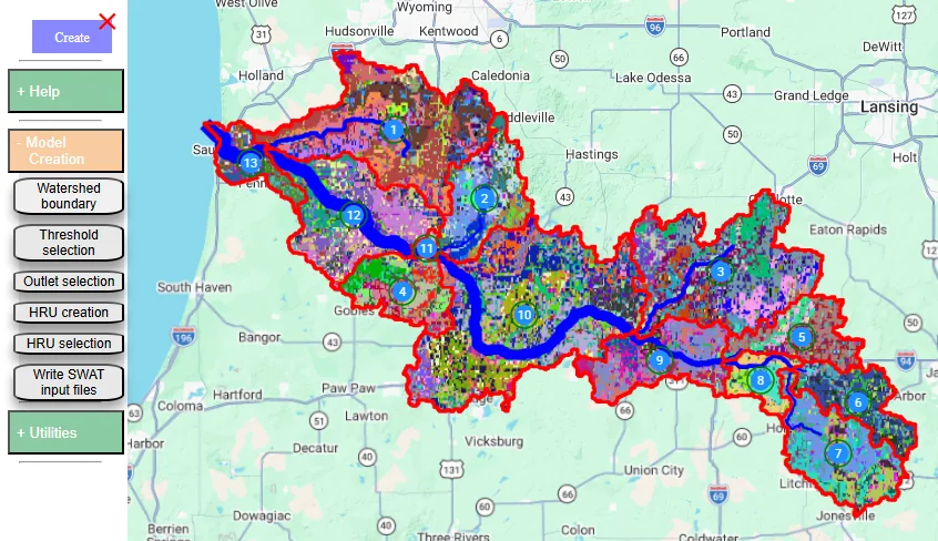
Watershed, subbasins, stream network, snapped outlet, land use, soil, HRUs — rendered as live textures on an interactive 3D terrain. Reveals where the action is spatially.
The system water balance Sankey is the watershed's hydrologic fingerprint — a complete quantitative picture of where water came from, what happened to it, and where it went. The values are real outputs from your SWAT simulation. Learning to read it is the single most useful skill for SwaNET work.
Inputs · Processes · Outputs
Water enters on the left — rainfall, snowmelt, initial soil moisture, irrigation. It passes through land-surface processes in the middle — evapotranspiration off the top, infiltration and percolation downward, runoff into the stream network. It leaves on the right — discharge out of the watershed outlet, deep aquifer storage, reservoir outflows. The widths of the bands are proportional to the volume of water moving through each pathway.
Inputs = Outputs ± ΔStorage
A watershed obeys conservation of mass: water in equals water out, plus or minus any change in storage. The Sankey makes the books visible. Note the small "Overland error" band — that's the model's residual closure error. A few percent is normal numerical drift; a large residual suggests configuration trouble. The Sankey lets you check the books at a glance.
What the proportions reveal
ET fraction — humid-temperate watersheds typically return 50–70% of precipitation to the atmosphere; arid systems return 80–95%. Runoff vs baseflow — flashy urban systems are runoff-dominated; groundwater-fed rural systems are baseflow-dominated. Deep percolation — high values mean recharge to regional aquifers, important for groundwater sustainability questions.
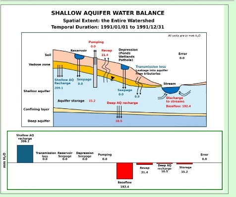
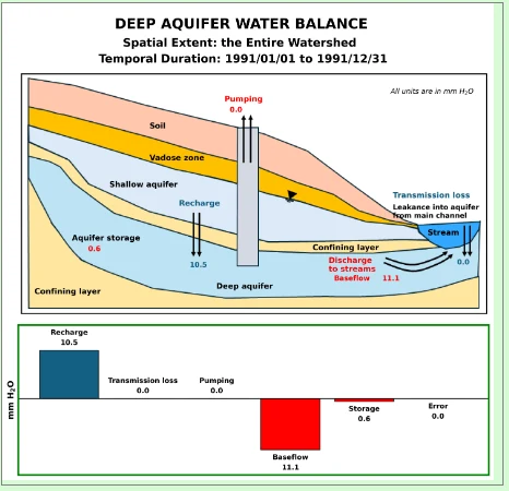
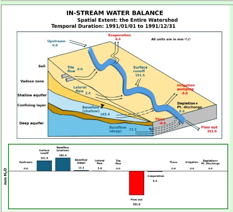
Beyond the system Sankey, SwaNET's drop-down menus let you inspect the water balance at four conceptual reservoirs. SWAT's strength is that it tracks water through each of these compartments separately — and SwaNET makes the books for each one visible. The values are pulled live from your simulation.
The first model runs on defaults — no observed data yet. The next four steps bring in real measurements from USGS or the Government of Canada monitoring networks and overlay them on the simulated time series. This is where you start seeing where the model gets the watershed right, and where it doesn't.
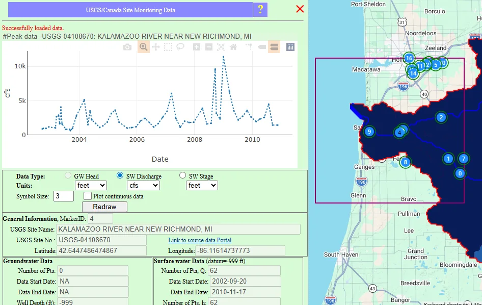
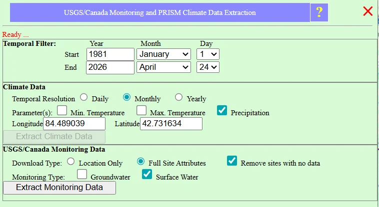
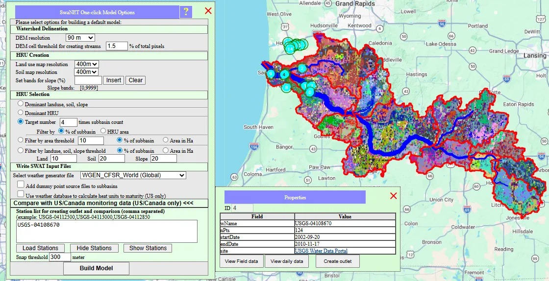
SwaNET's Utilities menu provides direct access to the USGS National Water Information System and Government of Canada monitoring networks. Draw an extraction area near the watershed outlet, configure the pop-up, and extract.
In the pop-up interface:
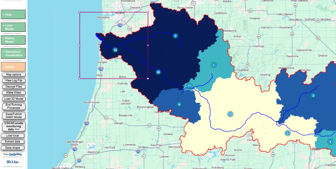
Once extraction finishes, stations appear as numbered markers on the map. Click any marker to view its time-series streamflow and stage data.
You're not starting over — you're loading your earlier project to refine it with finer-resolution data and observed-streamflow comparison.
Two targeted refinements: a finer DEM resolution for the watershed delineation, and a real USGS gauging station as the model outlet — so simulated and observed streamflow are at the exact same point.
Once the updated model finishes, you'll see the typical outputs again — 3D watershed visualization, water balance charts — but now the observed streamflow data is added to the time-series chart, overlaid on simulated streamflow.
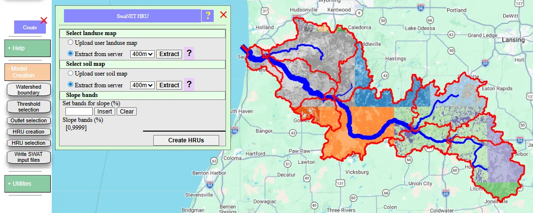
Higher-resolution land use and soil maps, plus a different HRU selection methodology. Two more steps, and you have a second model to compare against the first.
Load the latest project again. Navigate into HRU creation. Choose finer-resolution land use and soil maps, then change the HRU selection methodology.
Follow the on-screen interfaces to:
The updated results appear in the same display — but now you have two models to compare.
Resolution and HRU strategy are two dimensions of refinement. SwaNET keeps three more available in the same framework — weather data, subbasin-level edits, and model calibration. Every refinement runs through the same one-click model-building and visualization environment. No export. No re-import.
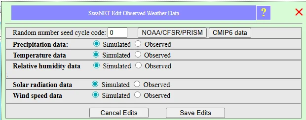
Add observed weather data instead of the synthetic generator. Different rainfall regimes, real station records, climate scenarios.
Change land use, soils, slope for a single subbasin. Edit point sources and discharge data. Test localized scenarios — a single farm, a single development.
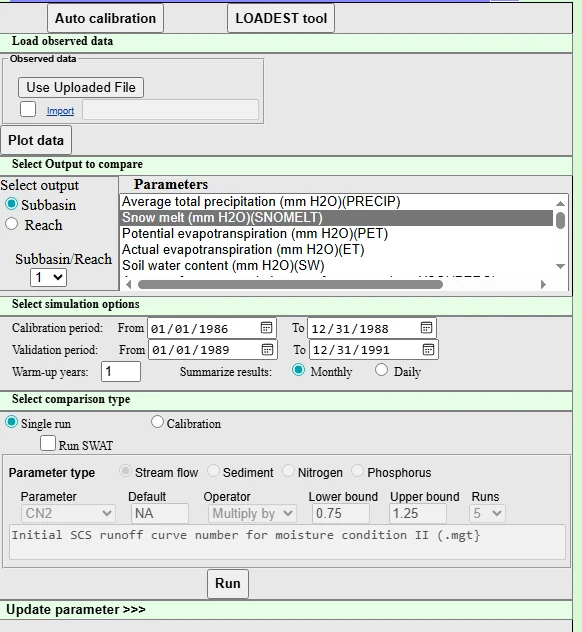
Adjust parameters to match observed streamflow more closely. One parameter at a time, or global calibration via a genetic algorithm.
The base enables. It never constrains.
You have built a watershed model in one click, read its hydrologic signature, compared it to observed streamflow, refined the resolution and HRU strategy, and identified three more refinement paths — all inside SwaNET, all in the same iteration loop. Time spent on data assembly: zero. Time spent on what matters: all of it.