When the calculations are complete the solution is presented as a contour plot such as shown in Figure 20. The continuous lines are the hydraulic head contours. The arrows are the macroscopic fluid velocities, which show the direction and magnitude of the groundwater velocity. The length of the arrow is proportional to the magnitude of the velocity.
Let’s see what information the model output provides. Recall that, by default, all lateral boundaries are ‘no flow’ so water does not leave or enter the model through lateral boundaries, and water only leaves the model through surface seepage where the head is greater than the land surface (see Section 3.1). Examination of the computed head contours (the wavy black continuous lines) reveals the water table surface. The easiest way to conceptualize the meaning of these contours is to draw the analogy with the elevations on a topographic map. Groundwater moves in a direction orthogonal to the water level contour lines. The arrows represent this flow pattern. The convergence of groundwater flow to major surface bodies is obvious.
The other factor at work in creating the observed solution (water level contours) is the aquifer thickness. The component of groundwater flow in the horizontal direction is directly proportional to the thickness of the aquifer. The product of thickness times hydraulic conductivity is called the transmissivity. So, where the elevation of the ground (water-table surrogate) is highest, the transmissivity is the highest because that is where the aquifer is the thickest (recall that in this basic model, the hydraulic conductivity is constant - even though in reality K is very variable - and the bottom elevation is a constant but the land surface is spatially variable). Since Darcy’s law tells us that groundwater flow is proportional to the hydraulic gradient and the proportionality coefficient is the hydraulic conductivity (in this case the transmissivity), we would expect the smallest gradient where the transmissivity, and therefore the aquifer thickness, is largest. This is reflected in the lower gradient around topographic highs (located near the center of the model). Of course, if we utilized a spatially-variable bottom aquifer surface and/or a spatially-variable hydraulic conductivity input, the output (and our interpretations) becomes more complicated.
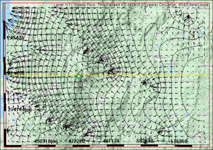
Figure 20: Computed and interpolated hydraulic head contours and groundwater velocities.