We are now ready to simulate in transient mode. Clicking on SIMULATE yields the familiar warning prompts; click OK and you will initiate the calculation. As the simulation is running, at the top of the plot you will see the elapsed simulated time (real elapsed time, not computer simulation time) and you can see the plot changing in response to the time-varying pumping rates (see Figure 83). Note how the contour lines around the well change in response to the time-varying pumping rates. In some cases, it might be difficult to notice the changes because the simulation takes place rather quickly on the computer so the simulated results at different timesteps may pass quickly. In addition, the results may not change much over each time step, so the outputs for different time steps may seem pretty much the same.
Just like steady-state simulations, it is possible to view the results in Chart view by clicking Analysis Tools, Analysis, then Display Charts. The familiar graphics will appear, but you will notice that some of the charts update as the simulation proceeds forward. For example, the mass balance chart will appear different at different time steps because of the time-varying pumping rates. If a monitoring well has been added to the model (see Section 5.4) a time-series head and/or concentration plot will be updated as the simulation proceeds.
At any point, you can pause the simulation by clicking Pause under Simulation Tools. You can perform further analysis (e.g. draw a new cross-section), but when you are ready to proceed forward with the simulation, click Forward under Simulation Tools.
In some instances, we may be interested in the model results for a particular time-step. Or we have a simulation that takes a long-time to re-execute, but we want to display the previously solved results without waiting for another round of simulation. For these situations, we can use the MAGNET Post Analysis Tool, which is discussed in the next section.
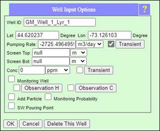
Figure 81: Enabling time-varying pumping/injection rates.
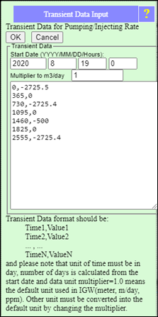
Figure 82: Assigning a transient pumping stress to the model.
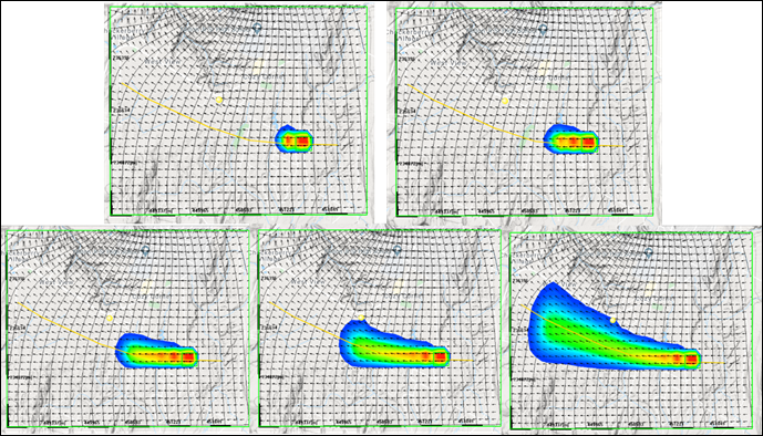
Figure 83: Simulation results for different time-steps of the unsteady model; note the changing contours near the pumping well.