The quick read — 90 seconds
- Three feature types layer on top of the domain and aquifer attributes: zones (polygons that override attributes locally), lines (rivers, drains, boundary conditions), and wells (pumping, injection, monitoring, observation).
- Zones have the same structure as the domain — a full Zone Attributes dialog with five tabs paralleling the Domain Attributes tabs. Where a zone is silent, the domain value applies. Zones also unlock scattered-point interpolation and T-PROGS (see Ch. 5 §5.10).
- Lines come in nine types, from simple prescribed-head boundaries to two-way stream-aquifer exchange. The most common: One-way Drain for small streams and ditches, Two-way Stream for larger rivers with bidirectional exchange.
- Leakance units follow geometry: rivers (lines) use m/day because channel width enters the formula; lakes and wetlands (polygons) use 1/day because area is already implicit. Same physics, different integration.
- Wells are defined by 13 fields — pumping rate (Q), location, screen interval, concentration (for injection), and flags for monitoring, observation, and particle release. A single well record can serve multiple purposes simultaneously.
6.1 The Three Feature Types
Features are what take a base model from "a region with generic aquifer properties" to "a specific site with real hydrogeologic elements." The three types serve different purposes and are drawn with different tools, but they share a common design: each is defined relative to the domain, and each can be edited through a dedicated Attributes dialog.
| Feature | Shape | Use for | Drawing tool |
|---|---|---|---|
| Zones | Polygons (rectangle or arbitrary) | Local attribute overrides — a region with different K, different bottom, different recharge; or a submodel domain; or a lake/wetland treated as a polygon feature | Draw Zone → ZoneRect or ZonePoly |
| Lines (polylines) | Line strings (multi-vertex) | Streams, drains, rivers, prescribed-head boundaries along a line, flux measurement sections | Draw Polyline → 9 type options |
| Wells | Points | Pumping wells, injection wells, monitoring wells, observation wells, particle release points | Draw Well |
From the solver's perspective, every feature you add becomes a modification to the solution at the cells the feature occupies. A zone changes per-cell K values (or whatever attribute the zone overrides) within its polygon. A polyline adds a boundary condition — prescribed head, flux, or head-dependent exchange — to the cells the line crosses. A well adds a source or sink term to a single cell. The drawing interface abstracts this away, but understanding it helps when you're diagnosing unexpected results: every feature exists in the grid, so features near cell boundaries may snap to one cell or another depending on the grid resolution.
6.2 Zones
Chapter 5 introduced zones as "refinement with teeth" — polygons where attribute values can override the domain's background values. This section covers the mechanics of creating and configuring zones.
6.2.1 Creating a zone
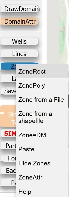
Choose the zone shape tool
In the Conceptual Model Tools panel, click Draw Zone. Choose ZoneRect for a rectangle or ZonePoly for an arbitrary polygon. Rectangles are faster; polygons match irregular natural features (lakes, geology contacts).
Draw the zone
For ZoneRect: click-drag to define the rectangle. For ZonePoly: click each vertex in sequence, then close by clicking the starting vertex or double-clicking.
Open Zone Attributes
Click inside the zone, or use the ZoneAttr button in the toolbar. A dialog opens with five tabs — paralleling the five tabs of the Domain Attributes dialog.
Set zone type and attributes
In the Zone Types section, choose what this zone represents: submodel domain, surface-water body (lake, wetland), source zone for transport, particle zone, etc. Then configure attributes in the relevant tabs. Values you specify override the domain's background values inside this polygon.
6.2.2 The Zone Attributes tabs
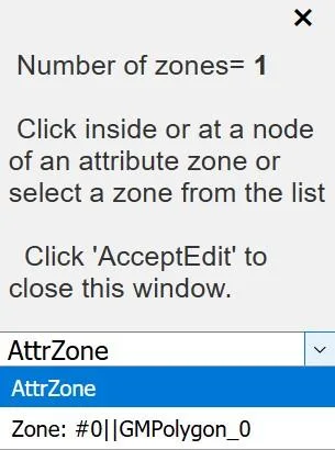
| Tab | Purpose | When you'd use it |
|---|---|---|
| Zone Types | Declare what this zone represents — submodel domain, surface-water body, source zone, particle zone, layer zone | Always — this is the first decision for any zone |
| Flow Properties | Override K, Sy, Ss, porosity, top/bottom elevation within the zone | Local refinement of aquifer attributes (e.g., a zone with different K based on local data) |
| Sources and Sinks Head Dependent | For polygon surface-water features (lakes, wetlands): stage, bottom elevation, leakance (1/day) | Adding a lake or wetland as a two-way head-dependent polygon feature |
| Sources and Sinks Prescribed | Prescribed-flux recharge, prescribed concentration sources, fixed flux-in | Localized recharge anomalies, contamination source zones |
| Display / Particles | Display settings for this zone; particle release configuration if it's a particle zone | Adjusting visualization or adding animated particles |
6.2.3 Common zone use cases
| Use case | Zone type | Key fields |
|---|---|---|
| Submodel for local refinement | Submodel Domain | Active checkbox only — inherits BC from parent |
| Lake or large pond (two-way) | Surface-water polygon | Stage, bottom, leakance (1/day), optional bathymetry |
| Wetland (can be one-way drain polygon) | Surface-water polygon | Stage = DEM surface, leakance (1/day) |
| Contamination source area | Source zone | Concentration (ppm), active start time, optional decay |
| Local geology zone with different K | Flow properties override | K value or scattered-point interpolation, zone porosity |
| Particle release rectangle | Particle zone | Particle count, forward or backward tracking |
6.3 Lines (Polylines)
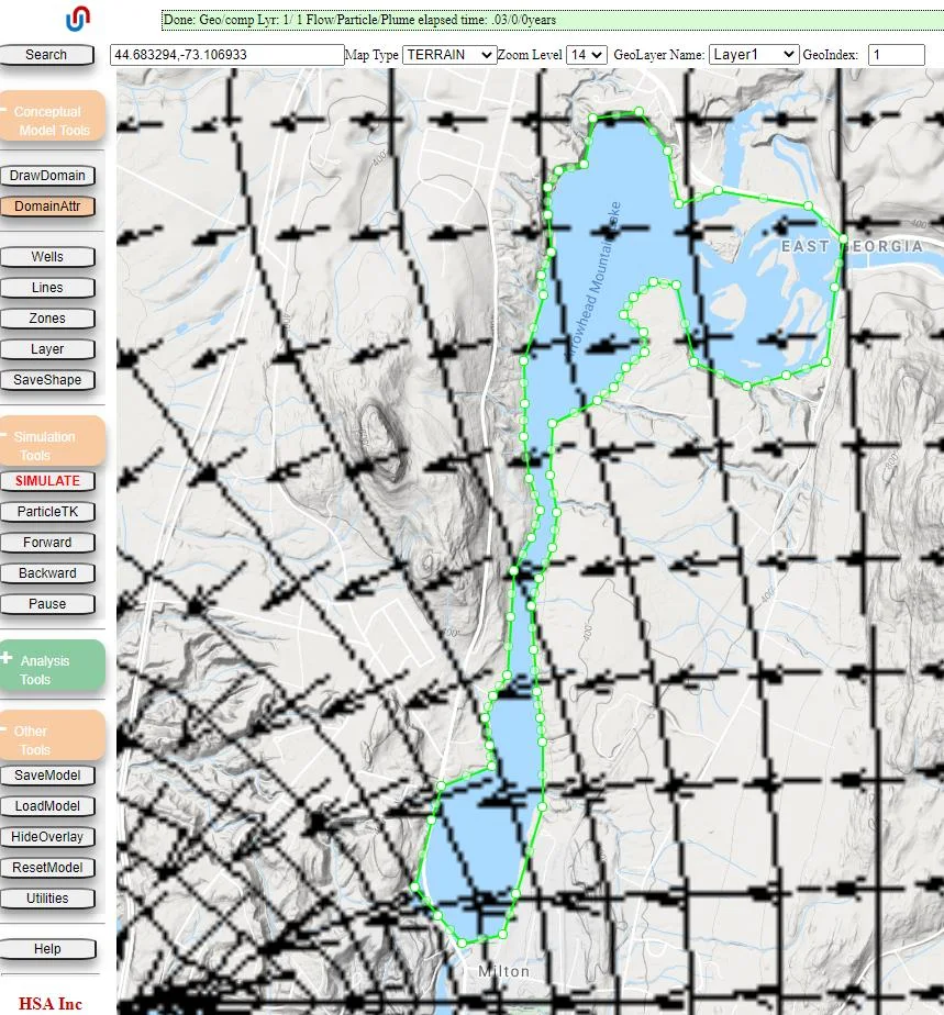
Line features represent one-dimensional elements — streams, drains, rivers, or boundary conditions along a line. The platform supports nine polyline types, each with a specific behavior. Choosing the right type is the most consequential decision when adding a line feature.
6.3.1 Drawing a polyline
Click Draw Polyline
In the Conceptual Model Tools panel, click Draw Polyline.
Trace the line
Click once at the starting point of your line feature (e.g., where the river enters your domain). Then click at each point along the line to add a vertex. Double-click at the final point to finish.
Configure the line type
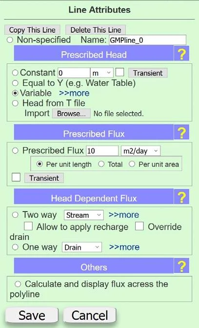
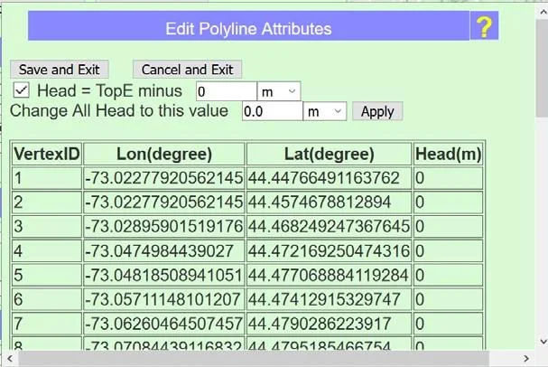
The Edit Polyline Attributes dialog opens. Select the polyline type from the dropdown (nine options — see next section), then fill in type-specific parameters.
6.3.2 The nine polyline types
Every polyline has a type that determines how the line interacts with the flow field. The nine types are:
| Type | Behavior | Typical use |
|---|---|---|
| 0 · None | Display only — no boundary condition applied | Annotation, reference lines, visual overlays |
| 1 · Prescribed Head (Constant) | Fixed head at every point along the line | Representing a large, stable water body as a constant-head boundary; regional head assumptions |
| 2 · Prescribed Head (Water Table) | Head equals the DEM surface elevation at each point | Representing topographically-controlled boundaries where the water table intersects the ground |
| 3 · Prescribed Head (Variable) | Head varies along the line as specified at each vertex | Rivers with changing stage along their length; head-varying boundary conditions |
| 4 · Calculate Flux | Measures flux across the line without imposing any condition | Quantifying groundwater discharge into a river, flux across a property boundary, zone-budget computation |
| 5 · Two-way Stream | Bidirectional head-dependent flux — water moves between aquifer and stream in either direction depending on relative heads | Larger rivers (3rd order and above), gaining-and-losing streams, river reaches where direction can change |
| 6 · One-way Drain | Aquifer discharges to the drain when head is above stream stage; no recharge from stream to aquifer | Small streams (1st-2nd order), ditches, drainage tiles, small ponds — features that consistently function as sinks |
| 7 · Prescribed Flux | Fixed flux rate (m³/day per unit length) across the line | Known inflow or outflow along a boundary segment; specified leakage from pipelines |
| 8 · Head from Transient File | Head varies with time, loaded from an uploaded CSV file | Transient simulations with time-varying stage at a stream or river gauge |
6.3.3 The most common choice — one-way drain vs two-way stream
Of the nine types, two account for the large majority of real-world use: One-way Drain (Type 6) and Two-way Stream (Type 5). Understanding when to use each matters enough to warrant a focused discussion.
As a rule of thumb mirroring IGW-NET's default behavior for explicit surface-water features: small rivers and ponds (1st-2nd order) should be one-way drains; larger rivers and lakes (3rd order and above) should be two-way head-dependent. The reasoning from Chapter 5 applies directly — smaller features function as sinks almost exclusively, so one-way is physically accurate and numerically safe. Larger features have genuine bidirectional exchange that matters hydrologically, so two-way is worth the extra configuration care.
6.3.4 Leakance for line features — the physics reminder
Chapter 5 §5.8.4 established the leakance physics; here's the practical application for line features:
leakanceriver = (Ksediment / thicknesssediment) × widthchannel
Units: m/day (flux per unit length of line). Typical values:
- Small streams, sandy beds: 1-5 m/day
- Larger rivers, typical alluvial beds: 5-20 m/day
- Heavily silted beds (poor connection): 0.1-1 m/day
- Gravel-bed rivers with good connection: 20-100 m/day
The default values IGW-NET provides are reasonable starting points. If the simulated exchange rates look off (compared to streamflow gain/loss observations), adjust leakance first — it's the most influential parameter for stream-aquifer interaction. Typical calibration multipliers stay within a factor of 3-10; needing more suggests the stream should be a different type (e.g., one-way drain instead of two-way stream).
6.4 Wells
Wells are point features that add pumping or injection stress, measure heads and concentrations, or serve as particle release points. A single well record carries 13 fields and can serve multiple roles simultaneously.
6.4.1 Adding a well
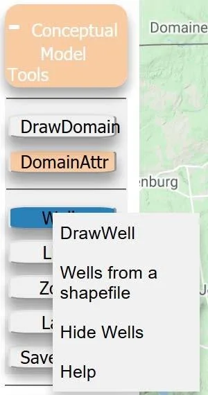
Click Draw Well
In the Conceptual Model Tools panel, click Draw Well.
Click the well location on the map
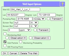
A single click places the well at that point. The Well Input Options dialog opens automatically.
Fill in the fields that matter
At minimum, enter a pumping rate (Q). Other fields are optional — you can leave name, screen interval, concentration, and flags at their defaults for a basic pumping well. See the field reference below.
Click OK to add
The well is immediately added to the model and will be included in the next simulation.
6.4.2 The 13 well fields
| Field | Type | What it does |
|---|---|---|
| NameID | String | Well identifier. Useful for keeping track of multiple wells; appears in result charts and reports. |
| Q_m3day | Float | Pumping rate in m³/day. Negative for extraction, positive for injection. Set to 0 for a monitoring well. |
| Lon, Lat | Float | Location in decimal degrees. Automatically set from where you clicked on the map; rarely edited directly. |
| isAddParticle | 0/1 | Whether particle tracking starts from this well. Used for wellhead protection analysis (backward tracking) and contamination impact analysis (forward tracking). |
| Conc_ppm | Float | Concentration of injected water (only relevant if Q > 0). Setting a non-zero Conc_ppm activates contaminant transport automatically. |
| isMonitoringWell | 0/1 | Whether the well reports simulated head and concentration over time at its location. Produces a breakthrough curve or hydrograph in the analysis tools. |
| ScreenTop_m / ScreenBot_m | Float | Vertical screen interval for layered models. Determines which computational layer(s) the well pumps from. |
| isMWProbs | 0/1 | Whether the well appears in probability-of-capture analysis (stochastic Monte Carlo contexts). |
| isSWPt / SWPtSlope / SWPtsWidth | Mixed | Surface-water point-source parameters — for wells that represent discrete surface-water recharge points. |
6.4.3 Common well configurations
| Configuration | Key fields | Used for |
|---|---|---|
| Pumping production well | Q = negative value (e.g., -500 m³/day); screen interval if layered | Water supply, dewatering, remediation extraction |
| Injection well | Q = positive value; Conc_ppm if injecting contaminated water | Aquifer recharge, waste injection, tracer tests |
| Monitoring well | Q = 0; isMonitoringWell = 1 | Reporting simulated heads and concentrations over time |
| Wellhead protection analysis | Q = realistic pumping rate; isAddParticle = 1; backward tracking | Delineating capture zones for drinking-water wells |
| Probabilistic capture zone | Q = pumping rate; isAddParticle = 1; isMWProbs = 1; stochastic mode | Wellhead protection under heterogeneity uncertainty |
You don't need separate well records for each role. A single well with Q = -500 m³/day, isMonitoringWell = 1, and isAddParticle = 1 functions simultaneously as a pumping well, a monitoring well (reports simulated head at its location), and a particle-release point. This is usually how real public-supply wells are modeled — they pump, they're monitored, and their capture zones are traced from the same location.
6.5 How Features Interact
Zones, lines, and wells are not independent — they can and do interact with each other and with the domain's default behaviors. Understanding these interactions saves hours of debugging unexpected results.
6.5.1 Zone overrides propagate to enclosed features
If a polyline or well falls inside a zone, the zone's attribute values apply at that feature's location — not the domain's. This matters most for K: a pumping well inside a zone with K override will draw from the zone's local K, not the domain's default. This is almost always what you want, but it's worth being aware of.
6.5.2 Streams override surface drainage
Chapter 5 §5.8 covered surface drainage discharge — the default mechanism by which any cell can discharge groundwater when the water table rises above the ground surface. When you add an explicit stream or drain polyline at the same location, the polyline takes precedence: the cells crossed by the polyline discharge through the polyline's leakance, not through the default surface drain. This is why adding explicit streams is a refinement, not a duplication.
At a cell where both DEM-as-drain and an explicit stream polyline are present, the explicit stream wins. The DEM surface-drainage default continues to operate at every other cell in the domain. This means you can add a few explicit features without worrying about the rest — the defaults fill in everywhere you haven't specified. See the Stream vs Drainage Precedence concept page for edge cases.
6.5.3 Wells and transport activate together
If you set a well's Conc_ppm to a non-zero value, you are telling the solver to inject water with that concentration. This automatically activates transport — the solver will now simulate how the injected contaminant moves through the aquifer. No separate toggle is required. This is the auto-detected transport behavior discussed in Chapter 12, and it applies equally to concentration sources in zones, polylines, and wells.
6.5.4 Features near domain boundaries
Features placed too close to the domain boundary interact with the default no-flow BC in ways that distort results. A pumping well within a cell of the boundary sees an artificial constraint on its capture zone. A stream that crosses the boundary sees head piling up against the no-flow edge. The fix is always the same: draw a larger domain, or move the features farther from the boundary. Buffering (Ch. 4 §4.3) prevents these problems before they start.
To go deeper
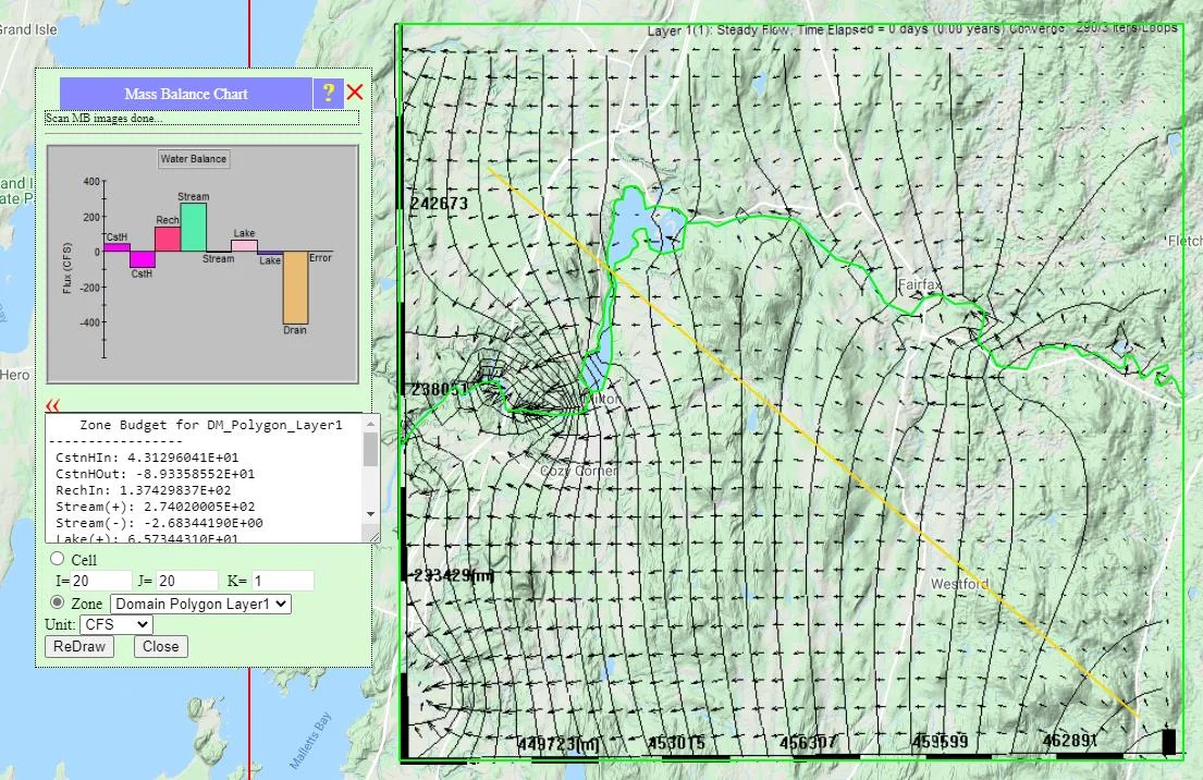
- Chapter 7 — Running the Simulation — next chapter. With features added, this covers what happens when you click SIMULATE.
- Chapter 12 — Contaminant Transport — more on how concentration sources in zones, polylines, and wells work.
- Chapter 12 — Particle Tracking — forward and backward particle tracking from wells and particle zones.
- Quick Tutorial 1: 2D Steady Flow — hands-on walkthrough including adding features.
- Concept: Stream vs Drainage Precedence — edge cases when streams and DEM-as-drain interact.
- Platform Reference: polylines — schema-level detail on all nine polyline types.
- Platform Reference: wells — complete well record schema.