§ 1 Model Philosophy
1.1 What is IGW-NET?
IGW-NET is a groundwater flow and mass transport model. It consists of two parts, the mathematical model
and a graphical user interface (GUI). The model is a computer program that solves numerically the equations that describe groundwater flow and mass transport. The GUI is a user-friendly interface that facilitates putting the information that the model needs into computer-readable form. It also organizes the input and output information in a format that is amenable to presentation in a graphical format.
1.2 Logical Structure of IGW-NET
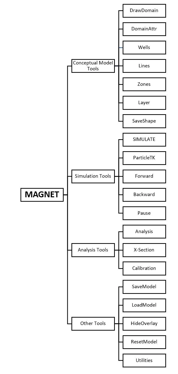
The model is presented to the user through a series of windows. The windows, in turn have sub-windows that include list boxes and drop-down lists. List boxes are passive in the sense that they provide a series of options that are always visible. Drop-down lists are activated and become visible only when a selection is made in a list box. In the Appendix the complete logical structure of the IGW-NET interface is laid out. The goal is to allow you to find any of the named buttons without having to search through the GUI structure to find them. It would be helpful if you turn now to the Appendix and scan the contents so you know what you can find and where you can find it when you need it. We will shortly, via an example, learn how these GUI elements work individually and work together. The IGW-NET model is essentially two integrated models, one to solve the groundwater flow equations and one to solve the mass (contaminant) transport equations. To solve the mass transport model, you require as (known) input the velocity of the groundwater. To obtain the velocity of the groundwater, you need the hydraulic head distribution (water level elevations). Using Darcy’s law and knowing the porosity of the geological materials through which the water is flowing and the head distribution, one can obtain the velocity of the dissolved species (such as salt or organic contaminants). So, there are three separate steps 1) solve the groundwater flow equations for hydraulic head, 2) solve Darcy’s law for the dissolved species velocity and 3) introduce the velocity into the mass transport equation and solve for the concentration. As noted, one objective of the GUI is used to translate known model information from a visual format such as a map into a series of numbers that are readable by a computer. A second GUI responsibility is to translate the numbers generated by the computer model into a visual format understandable to the user. In addition, the GUI can visualize computer commands such as printing, file saving, and file selection.
§ 2 Access to IGW-NET
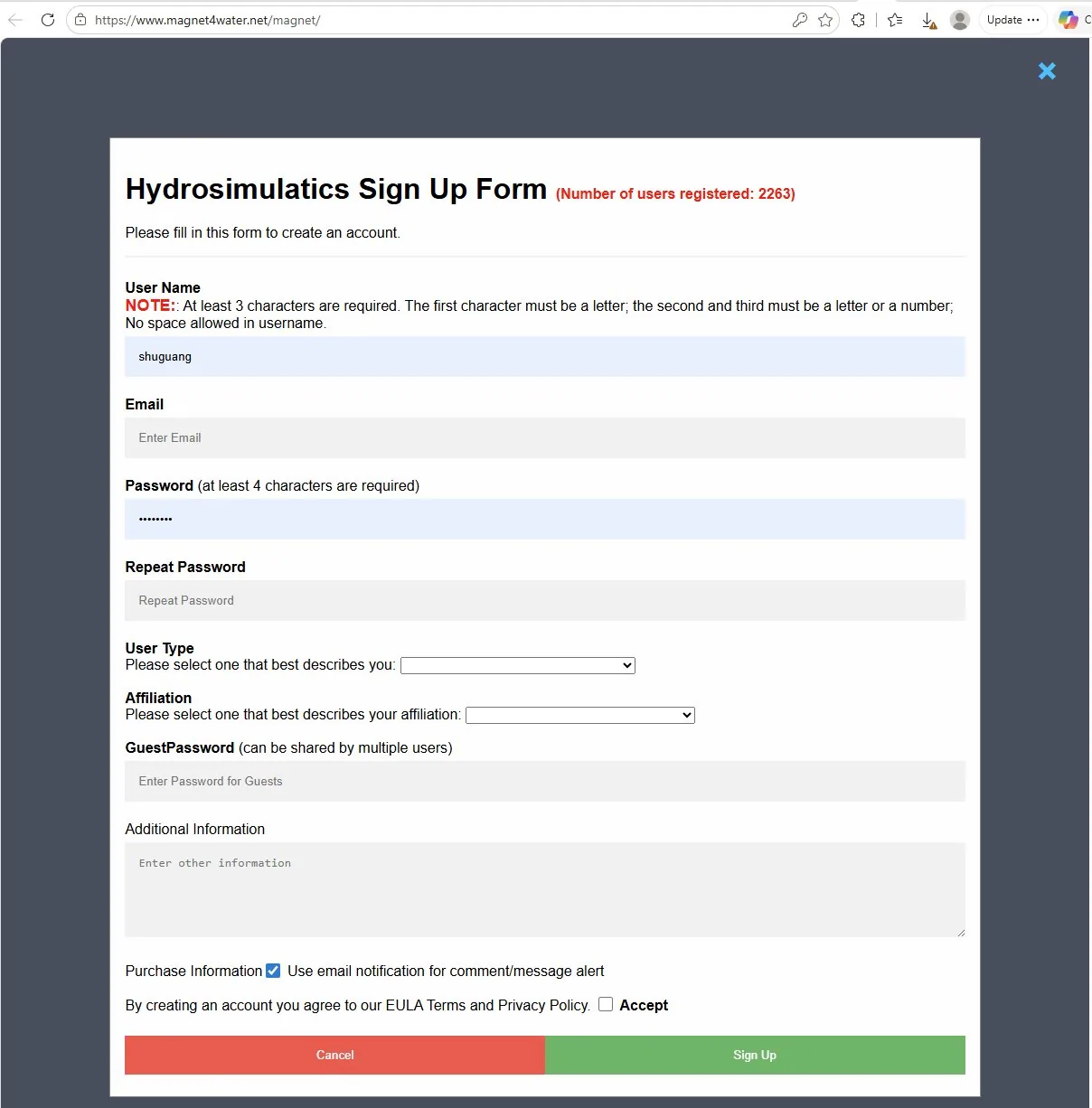
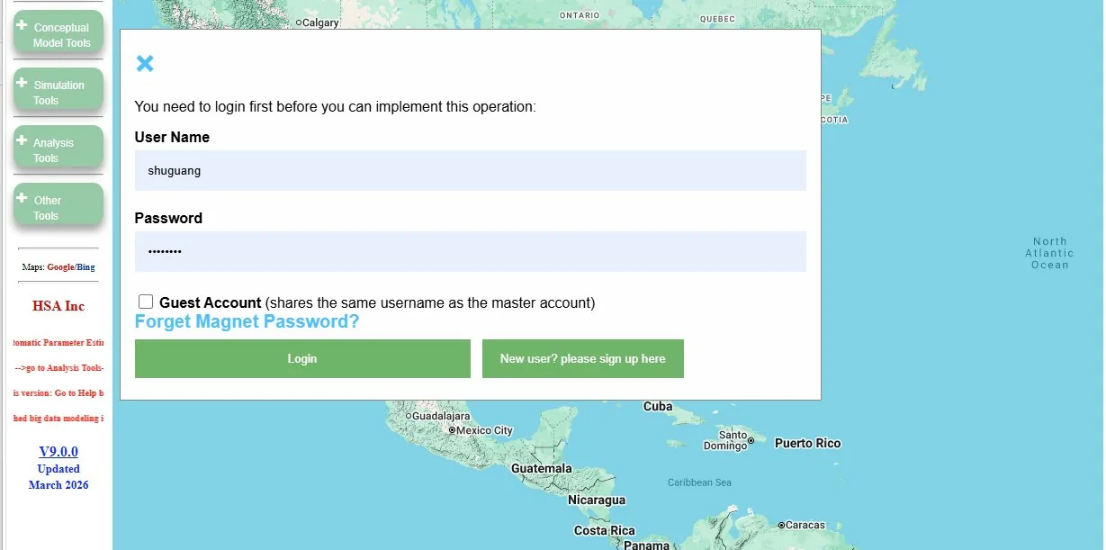
IGW-NET is accessed through the MAGNET4WATER cloud platform in a standard web browser such as Chrome, Edge, Firefox, or Safari. Begin from the MAGNET4WATER site, create or sign in to your account, and then launch IGW-NET from the platform entry page. An account is needed before running models so that simulations, model files, settings, and saved workspaces can be stored securely on the IGW-NET server.
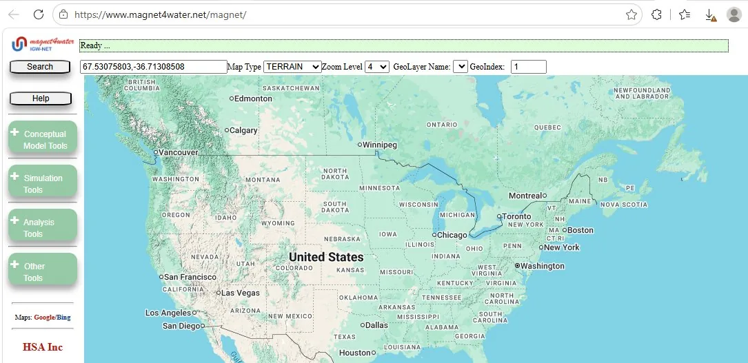
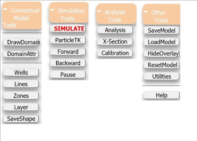
For a new user, select Sign Up or Create Account, complete the registration form with your name, email, password, and organization or affiliation, then sign in. After login, open the platform launchpad and choose Groundwater / IGW-NET. The IGW-NET workspace opens as a map-based modeling environment with tool groups for domain drawing, aquifer attributes, simulation, analysis, file operations, and help.

§ 3 Setting Up a Basic Flow Model
The philosophy of modeling with IGW-NET is to very quickly set up and simulate a basic model - utilizing a complete set of default input values/datasets, default simulation settings, etc. – so that you can immediately get a sense of the “big picture” through built-in visualizations and chart analyses created “on the fly”. The basic model gives a screening-level prediction of flow patterns that can be improved by representing more details, adding more data, or changing the conceptual model based on the objectives at hand and the experience of the modeler. The following sections explain the sequence of steps needed to set up, simulate, and visualize/analyze a basic model in IGW-NET. Subsequent sections explain how incrementally add more and more details to the basic model.
3.1 Lateral Boundaries of the Model
Observe in Figure 5 the four green buttons on the left side of the modeling environment. Each of these yields a list box upon clicking. Figure 6 shows the contents of each List box. In setting up our model, we will normally begin with the top button in the left-most drop-down list. The DrawDomain button will be used to do just that, draw the domain or area of interest of our model (see Figure 7) . Since we first need to draw the domain,we click on this button on obtain the following four options. The first will allow us to draw a rectangular domain very efficiently. This is the easiest choice and the one we will use. The DomainPoly option is an important alternative. It allows us to draw any polygonal area as the domain for our model. The next two, DM from a txt File and DM from a shapefile allow us to bring in information about our domain in a computer file when it is known, rather than actually drawing the domain with the mouse. Since the map shown Figure 5 is at a very small scale we need to enlarge the scale to identify the area of interest for our model. Let’s see how we move around this world map and change its scale. As long as the hand is visible over the map, double clicking and moving the hand moves the map. If you use the ctrl key and scroll, the map changes scale. If you left click the window while moving the hand will move the map. We will first move the map to the general area we want to use for our model and then magnify the model to focus on the primary area of interest. We get the map shown in Figure 8.
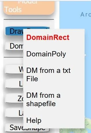
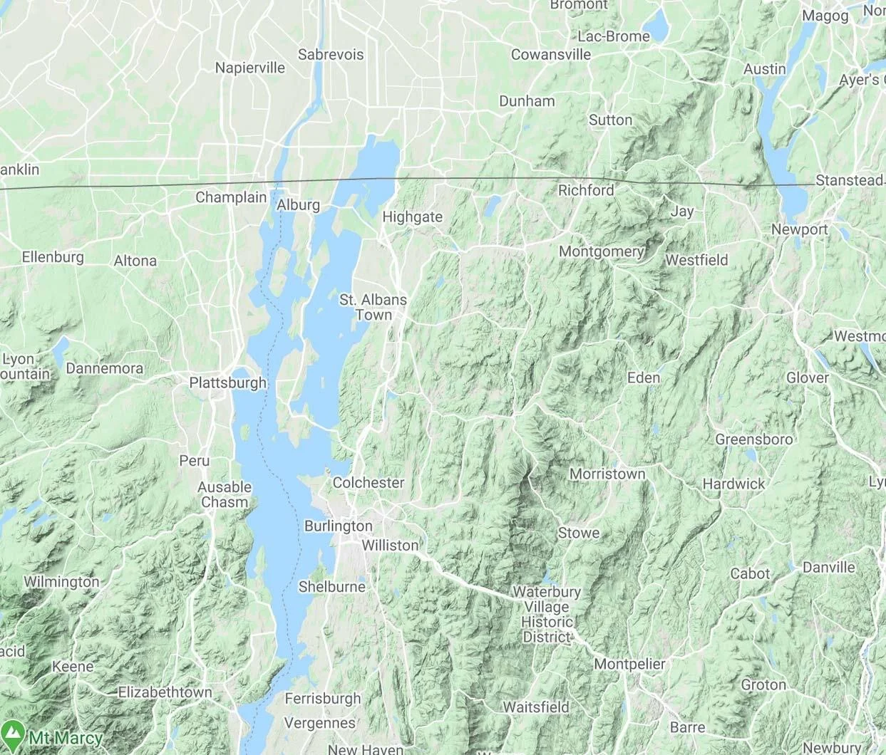
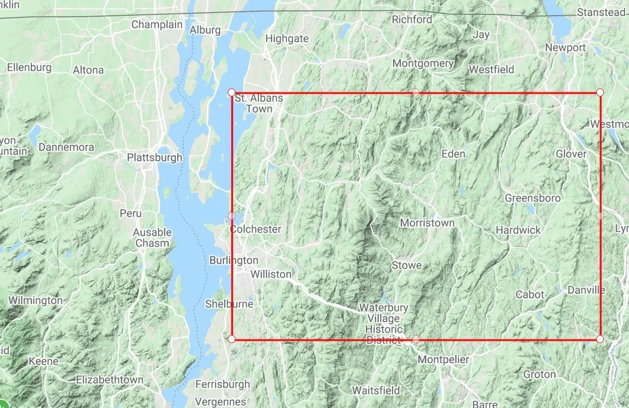
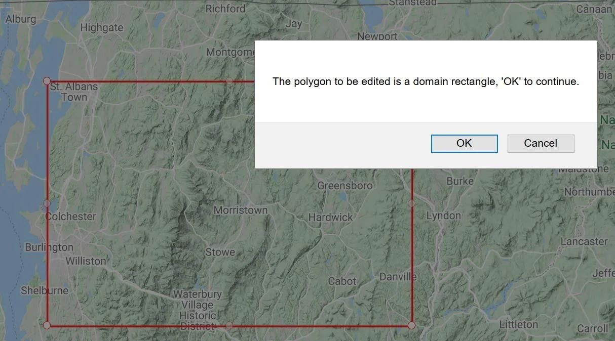
Next, we click on Conceptual Model Tools and then Draw Domain and finally on Domain Rect as shown in Figure 9. When you move the mouse over the map area, you will see your mouse turn into a large plus sign. Place the mouse on a corner of the domain you want to create, say, for example the upper left-hand corner (northwest corner). Click the mouse and then move the mouse to the location of the proposed rectangle that is furthest from the point you just created. In our case that could be the lower left-hand corner (southeast corner). When you click you mouse, the rectangle will be created. Note that there are four corner points on the rectangle that will allow you to adjust the size and shape of the rectangle. Also note that you cannot click too quickly; the clicks need to be done slowly, with a second or two in between so that IGW-NET (as a web-based platform) has enough time to react. The next time you click anywhere inside the model domain you will get window shown in Figure 10. Click OK to continue. You will be rewarded with another prompt (Figure 11) related to displaying display distances between vertices in the map display the next time you adjust the domain shape/size by dragging one of the vertices. Again, click OK. If you do this an undo button will appear next to it to reset the location to the previous position. Only the last position is kept in ‘IGW-NET’s memory’. The message will disappear. A second way to finalize the domain size and shape is to click the Conceptual Model Tools button and then click the SaveShape button. A third way is click on Other Tools and then on Utilities and finally on Geometry Locked. Both the 2nd and 3rd approach avoid the message prompts described in the previous paragraph. If you want to change your rectangle entirely go back to the DomainRect button and click it. The rectangle you just created will disappear and you start the process over. There is no universally applicable ’undo’ button in this program.
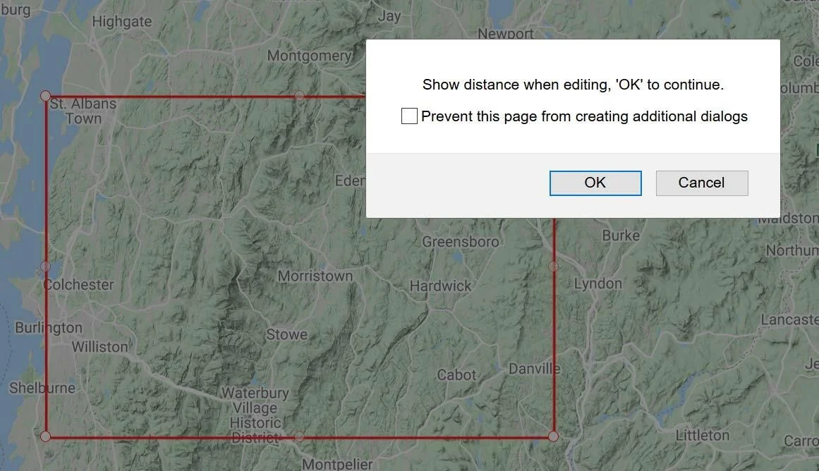
Along the lateral and bottom boundaries are considered “no flow” boundaries (the top surface is a different story – more on that below). In other words, there is no flux of groundwater across these boundaries. Unless the boundary is aligned with a groundwater divide (which is hard to identify, and which changes in response to changes to recharge or pumping, for example), there may actually be some flow across the model boundaries. Therefore, the basic flow model we are developing may not be very accurate near the boundaries. But we can make the model large enough so that the area of interest is far from the boundary so the impacts of the no-flow conditions can be eliminated/minimized. Later we will learn how to use the basic model to provide boundary conditions (flow information) for a smaller, nested submodel with more details (see section 5).
3.2 Aquifer Attributes
Now that we have specified the boundaries of our model (but not our boundary conditions) we can define the geometry and the hydraulic properties of the aquifer. This is done by accessing the Domain Attribute menu by clicking the Conceptual Model Tools button and then clicking DomainAttr (see Figure 12). When you click DomainAttr the button it changes color and you the Domain Attributes menu opens (see Figure 13).
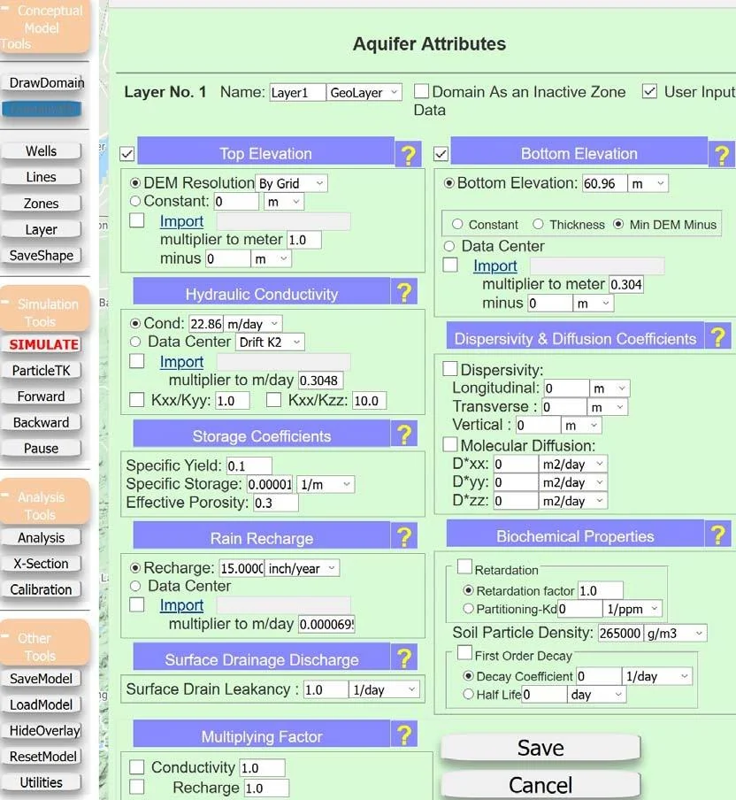
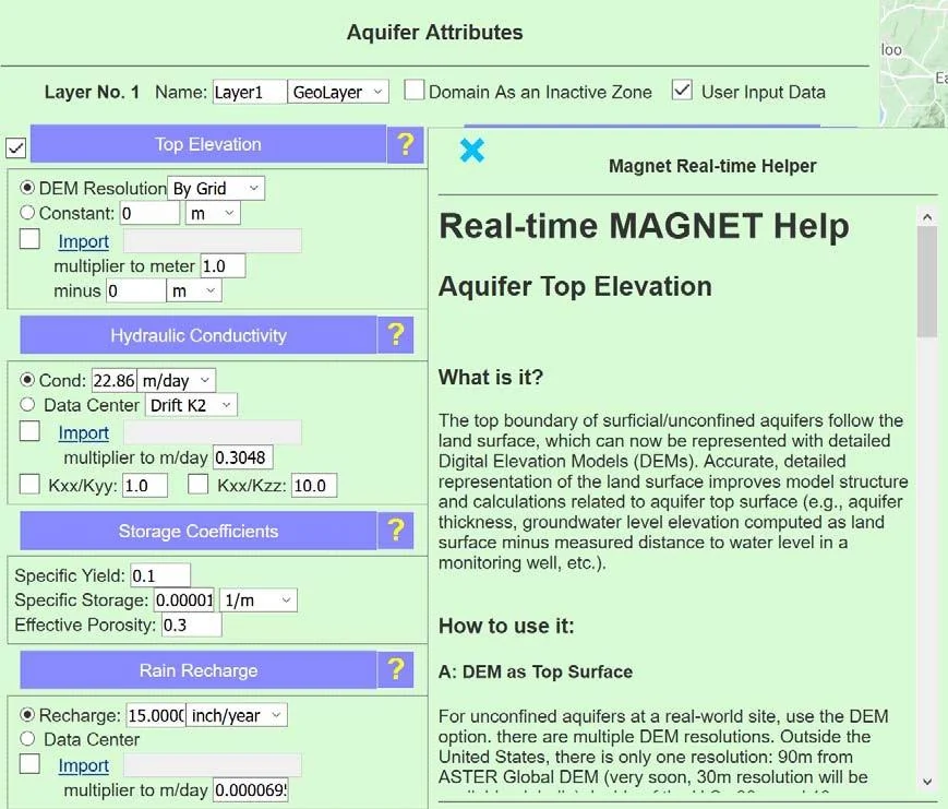
Here you see tabulated the various properties of the groundwater system that you can define. Default values are provided. These can be changed to meet the needs of your aquifer system. Some are familiar, such as hydraulic conductivity and storage coefficients that pertain to the groundwater flow calculation, and others are needed for the mass transport capability such as dispersivity, diffusion coefficient, and biochemical information. Also included is information on flow into the system within its boundaries including recharge from rainfall recharge. Notice that at the top of this window there is a layer designation. It states that this information is pertinent to layer 1 which is a Geolayer, or layer that is defined to accommodate geological properties (IGW-NET can accommodate multiple vertical layers – see section 7). It is also possible to define layers within a geolayer that are used to increase the simulation accuracy in the vertical direction (again, see section 7). Notice that there are question marks at the end of each data entry definition, for example next to the Top Elevation heading. If you click one of these question marks you will open a new window that give an explanation of the meaning of the. designated term, in this case Top Elevation.
3.2.1 Aquifer Elevations
Top Elevation An example Help page for Aquifer Top Elevation is provided in Figure 14. It is worth noting that in the Aquifer Top Elevation description is mentioned the fact that, while the top elevation of the model can be provided as a single number, it is also possible to define it as a surface, that is to say that different values
are provided in different areal locations. The database for this is designated as a Digital Elevation Model or DEM and provides a better representation of reality. This is used in this test dataset. IGW-NET uses data that is processed and stored at different resolutions. The code automatically extracts the appropriate DEM based on the grid size of the model. This is done by default1. In addition to the DEM from the MAGNET Data Server, users can add spatially -variable data layers to represent the aquifer top elevation by importing a raster format file. Bottom Elevation The bottom of the elevation can be represented in several different ways. The default treatment is the simplest: a constant elevation for the entire aquifer bottom surface, which is calculated as a prescribed value below the minimum DEM elevation within the model domain. The bottom elevation can also be calculated by prescribed a constant aquifer thickness, following the variable land surface; or, the user can use spatially-variable thickness/elevations available from the MAGNET Data Server, or by importing their own raster file. The models presented in this document apply the default treatment: constant elevation calculated from minimum DEM minus 60.96m (200ft).
1 The data network page on magnet4water.net gives a current listing with details of all big-data inputs offered on MAGNET.
3.2.2 Aquifer Properties
Hydraulic Conductivity The simplest treatment for defining the hydraulic conductivity (K) of the aquifer is to assign a single, effective value, which is what is presented here (22.86 m/d or 75 ft/day). But other options are also available. It is possible to upload a raster file with spatially-varying K; or you can use spatially-variable K data available from the MAGNET Data Center Serve. Zone features (polygons) can be added within the model to represent local heterogeneities with a local K value different from the domain K. With zones, you can also use scatter points for spatial interpolation of K, or you can generate a random K field defined by a group of statistical parameters. Adding zones and defining their attributes is covered more in the Sections 5 and 6.
Porosity To calculate the seepage velocity – or the velocity at which the groundwater is moving – porosity must be prescribed to account for the actual open space available for the flow. By default, a single value is used across the domain (0.3 or 30%); but like K, you can use zones to represent local heterogeneities (localized effective values or interpolation of scatter points) Storage For transient simulations of groundwater systems, the elasticity of the aquifer needs to be defined. The elasticity is not due to the elasticity of the individual grains that make up the aquifer, but rather reflects primarily the rearrangement of the individual grains as the fluid pressure in the aquifer changes. There is also an elastic effect due to the elasticity of water (water expands a little with a decrease in pressure), but it is minor relative to the impact of grain rearrangement. In IGW-NET, we represent this elasticity in terms of aquifer storage (specific yield or specific storage). By default, a specific yield of 0.1 and a specific storage of 10-5 m-1 is applied through the model domain; but again, you can use zones to represent local heterogeneities (localized effective values or interpolation of scatter points).
3.2.3 Aquifer Sources and Sinks
The basic model using default settings can be described by an aquifer water balance where recharge (input of water) is countered by surface seepage to gaining water bodies (loss of water). Other sources or sinks (for example, extraction and injection wells, losing streams or rivers, etc.) can be added to the model incrementally. Recharge from Rainfall Groundwater recharge is the entry of water into the saturated zone at the water-table surface. In IGW-NET, recharge is treated as a model input of specified flux [L/T] that is constant in time. (Time-varying recharge can be assigned using zone features). Here, a single value (15 in./yr.) is applied through the model domain (default setting), but you could also use the spatially-variable recharge raster available from the IGW-NET data server or your own raster file of recharge. Surface Drainage to Rivers, Lakes, and Wetlands / Springs IGW-NET “automatically” captures the effects of major drainage features (lakes, streams, rivers and
wetlands) that control prevailing flow patterns under natural conditions. This is done through intelligent
use of the aforementioned High-resolution Digital Elevation Models (DEMs) that provide aquifer top information essentially “everywhere” on earth. The default treatment in IGW-NET is to calculate, during the simulation process, instances where the groundwater head exceeds the land surface elevation, i.e., where gaining rivers / lakes / wetlands are found, allowing groundwater to leave the aquifer as a sink of water (i.e., groundwater is lost as surface seepage). This approach captures the spatially-distributed aquifer drainage effects of groundwater to gaining surface water bodies (groundwater-fed lakes, streams, wetlands, and springs) as part of the robust solution process, as the surface water stages (elevations) are embedded in the high-resolution DEM datasets used for assigning the aquifer top elevations. The ease with which water can drain from the aquifer to the surface is controlled by a parameter called Surface Drain Leakancy, a factor representing the hydraulic conductivity per unit thickness of the land surface. The leakancy can be adjusted or fine-tuned to better reproduce the observed surface water network, e.g., if the leakance is too low, the flooded area will be large, and vice versa. The input field for this parameter is provided in the Aquifer Attributes tab of the Domain Attributes menu (see Figure 13). If you wish to “turn off” treating the entire land surface as a drain, and instead represent surface water bodies using conceptual features (zones and lines – see Section 5.3), you can set the Surface Drain Leakancy to zero. Losing surface water bodies (where the groundwater head is less than the water body’s stage), are not represented in this default treatment, but MAGNET users can add zone or line features to the model as lakes or streams to allow two-way exchange of water and/or stages that vary with time. IGW-NET also includes an Import Shapefile tool to add many streams/rivers, lakes and wetland features in this way, or users can automatically extract surface water features (lakes and streams) from the MAGNET Data Center and add them as conceptual features to the model.
§ 4 Simulation
4.1 Running the Model
The information provided in the Aquifer Attributes window is adequate to run a model, provided that boundary conditions are provided around the perimeter of the model. As previously mentioned, for the initial, basic model such as we have so far, the boundary conditions are assumed to be no flow. Any submodel or child of the parent model (the one we are working with now) will assume fixed hydraulic head boundary conditions that correspond to the computed head values obtained using the parent model along the child model boundary (see subsection 5.1). The head values that are calculated to be higher than the land surface are assumed to be seepage locations the model. For the case of a steady-state (time
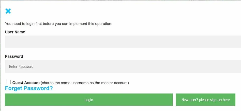
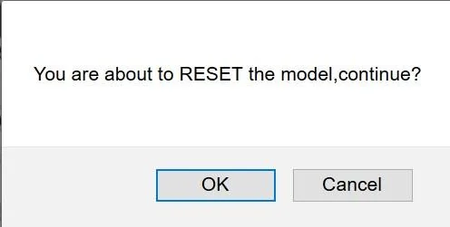
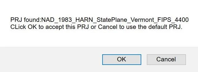
independent) model we have specified the minimum amount of information needed for simulation (solution of the groundwater flow equations). To simulate the behavior of the above-defined mode,l we simply press the SIMULATE BUTTON which is revealed by clicking on the Simulation Tools button revealed in Figure 15. The result of this action is presented in Figure 16. You must now use the information you provided earlier when you signed up to fill in this window. Once this is successfully completed, you click Login and a confirmation prompt will appear (Figure 17). A message regarding resetting the model and another the projection system to be used for simulation and mapping will appear next (Figure 18) and you click OK to each to proceed. Then your submission for simulation begins. At the top of the window you will see the progress of your simulation. One such message is shown in Figure 19.

4.2 Presentation of Results
4.2.1 Plan View Map Display
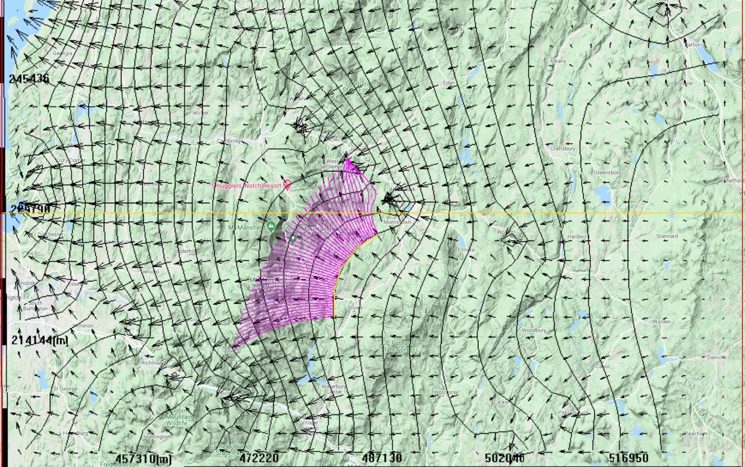
When the calculations are complete the solution is presented as a contour plot such as shown in Figure 20. The continuous lines are the hydraulic head contours. The arrows are the macroscopic fluid velocities, which show the direction and magnitude of the groundwater velocity. The length of the arrow is proportional to the magnitude of the velocity.
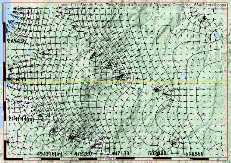
Let’s see what information the model output provides. Recall that, by default, all lateral boundaries are ‘no flow’ so water does not leave or enter the model through lateral boundaries, and water only leaves the model through surface seepage where the head is greater than the land surface (see Section 3.1). The convergence of groundwater flow to major surface bodies is obvious. The other factor at work in the observed solution is the aquifer thickness. The ability of water to flow horizontally in the subsurface is directly proportional to the thickness of the aquifer. The product of thickness times hydraulic conductivity is called the transmissivity. So, where the elevation of the ground (water-table surrogate) is highest, the transmissivity is the highest because that is where the aquifer is the thickest (recall that in this basic model, the hydraulic conductivity is constant - even though in reality K is very variable - and the bottom elevation is a constant but the land surface is spatially variable). Since Darcy’s law tells us that groundwater flow is proportional to the hydraulic gradient and the proportionality coefficient is the hydraulic conductivity (in this case the transmissivity), we would expect the smallest gradient where the transmissivity, and therefore the aquifer thickness, is largest. This is reflected in the lower gradient around topographic highs (located near the center of the model). Of course, if we utilized a spatially-variable bottom aquifer surface and/or a spatially-variable hydraulic conductivity input, the output (and our interpretations) becomes more complicated.
4.2.2 Flow Pathlines
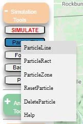
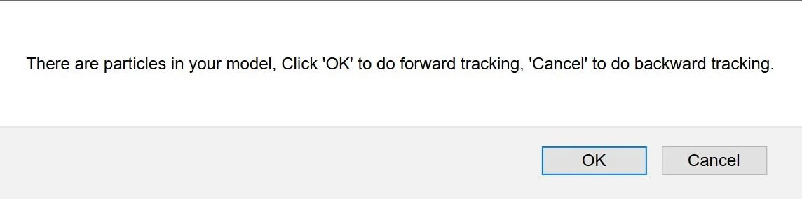
The simulated head and velocity distributions can be used to visualize groundwater pathlines. A pathline is the trajectory that individual fluid particles follow in a steady-state flow field. We will next calculate pathlines for mathematical particles that we will locate in our model. IGW-NET will allow you to introduce these particles in a number of ways, e.g. placing them as individual points, within a polygon or around a pumping well. Given our existing flow model, the first step in computing and plotting path lines is to click on Simulation Tools and then ParticleTK (see Figure 21). You can add particles along a drawn line, or inside of a rectangle or polygon added to the map display. We will add a particle line along a head contour near the center of the model where flow is diverging. Click the ‘ParticleLine’ option. A large “plus sign” (+) will appear on your model and you can trace the line segment along which to place your particles. The trace will be made
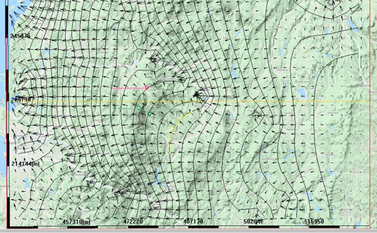
up of connected dots whose positions can be edited with click-drags. Each new click in the map display will produce a dot. The end result appears in Figure 22. Then re-submit the model for simulation, accept the projection system, and click on OK and you be asked whether you want forward or backward tracking (Figure 23). Backward tracking traces a path from where the particles you have defined came from in the past. Forward tracking in contrast defines where they will go in the future. We wish to do forward tracking, so click OK. As the model calculates the time evolution of the particles, the window that contains the figure is continually updated so it is possible to observe the changes over time of the groundwater hydraulic head and the movement of the particles. The results after many simulation years is shown Figure 24. Note that some of the pathlines are longer than others. These represent longer distances traveled by some particles compared to others over the simulation period. The longer pathlines are found in areas where contours are closely spaced together, indicating larger head gradients and larger resulting groundwater flow velocities.
4.2.3 Cross-sections
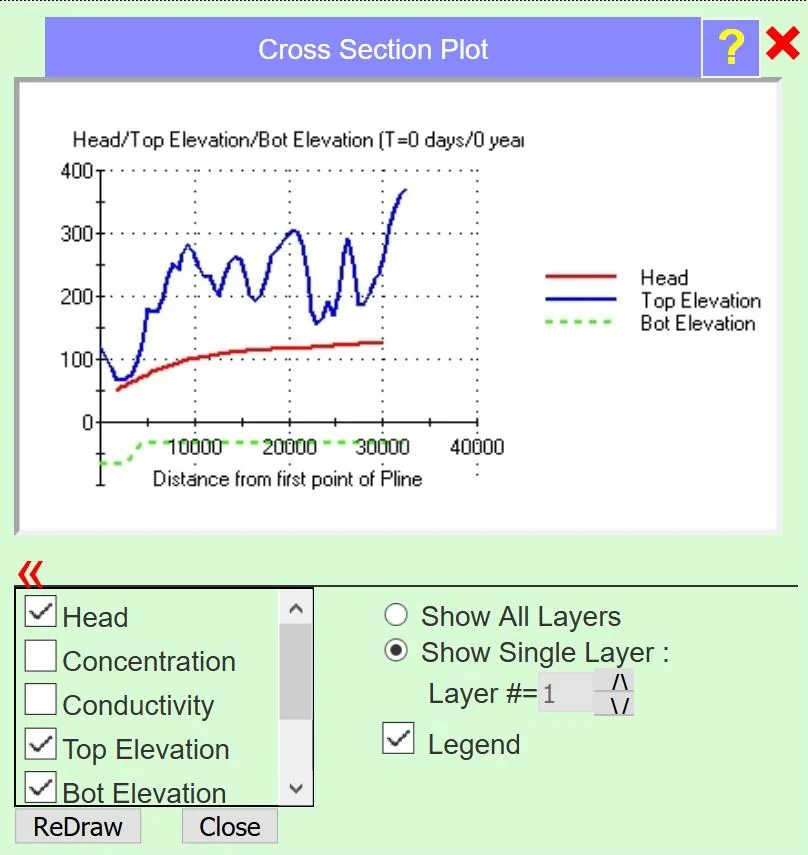
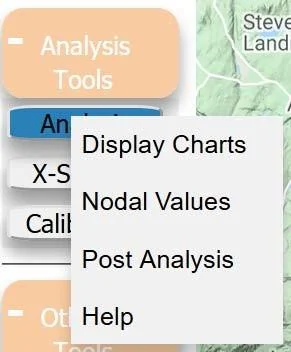
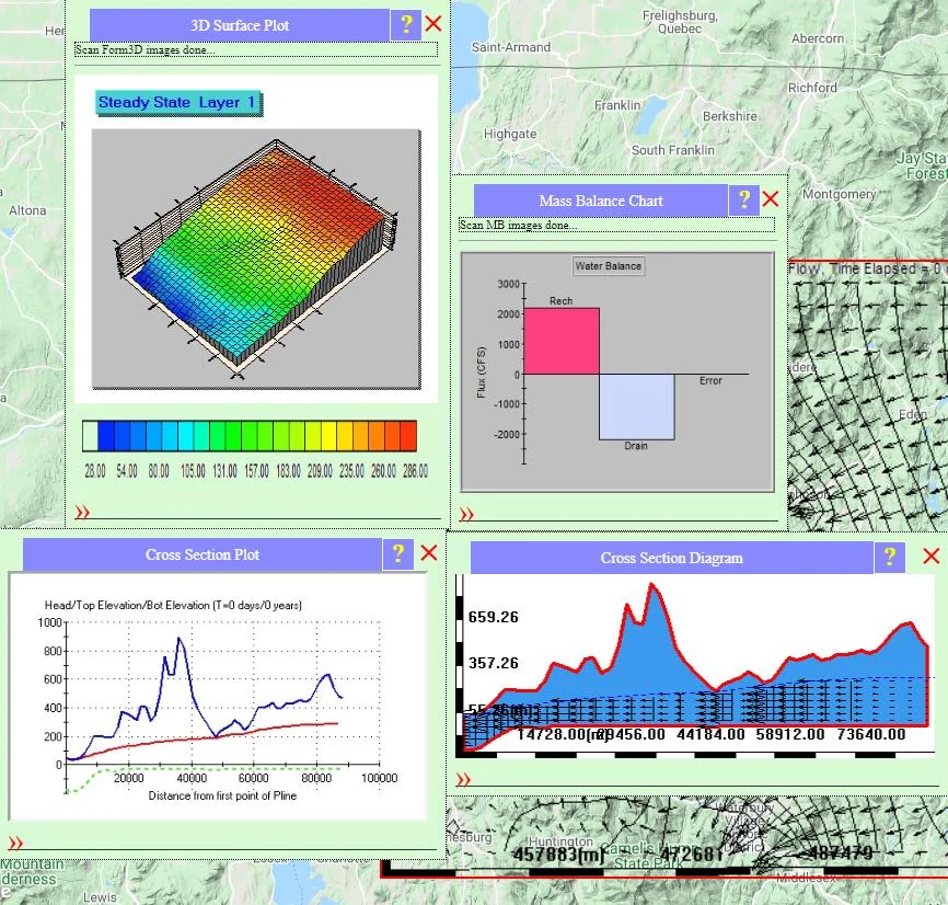
You may have noticed that when the simulation results are returned to the map display, there is a yellow line stretching across the center of the model in the x- (west-east) direction. This is a cross-section that is automatically created when the model is solved. In fact, IGW-NET automatically creates a number of charts and diagrams useful for analysis of the model results. To access the cross-section results and other analyses, click the Analysis Tools button, click Analysis, then choose Display Charts from the list of options (see Figure 25). Four plots will appear as shown in Figure 26: a cross-section diagram; a cross-section plot; a water balance chart; and a three dimensional surface plot of the water table. The cross-section diagram shows the aquifer top and bottom elevations, the water table elevation, and flow velocities (vectors). The cross-section plot shows in a graphical format the top elevation, the water table solution (smooth red line) and the bottom of the aquifer elevation. Other options are available for plotting (e.g., hydraulic conductivity along the cross-section).
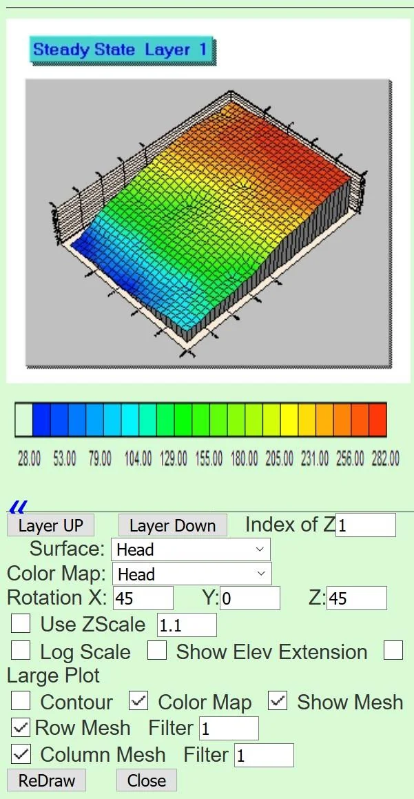
At any time, you can draw a new cross-section within the model domain. To do this we need to return to the analysis tools and select from them the X-Section button. When you click on the X-Section button, the cursor will become a large plus sign. Locate the plus sign at the beginning of the line you plan to use to represent where on the contoured map you wish to have your cross section drawn. When you complete drawing the line, you can click ‘SaveShape’. This re-creates the cross-section diagram and plot for the new cross-section. Note the chevrons (‘>>’ button) on the lower left of the various charts. Clicking on the chevron provides additional information regarding the content of the plot and how to modify it. As an example the chevron for the 3D Surface Plot yields the window shown in Figure 27. Here, for the first time we see reference to a mesh. The mesh is the assemblage of blocks that together make up the fabric of the computer model. The more blocks, the more precise and accurate is the model. Each block spawns one equation so the number of equations being solved in this model is the sum of all the blocks in the model.
4.2.4 Water Balance
A water balance (or water budget) like the one shown in Figure 26 reveals the amount of water moving into and out of the system (recall that, in the basic model, aquifer recharge is balanced by surface seepage). A water balance is automatically created for the model domain every time a model is submitted for simulation. Positive fluxes represent sources of water to the zone/domain, while negative fluxes represent sinks of water If you click the chevron of the Water Balance chart, you will see that water balance analyses can be conducted not only for the model domain, but also for any zone added to the model domain (see Flow Properties tab of the Zone Attributes menu) or a single grid cell of the model. You will also see that default
units are cubic feet per second (CFS), but users can change the units to gallons per minute (GPM) or cubic meters per day (m3/day) by using the drop-down menu next to ‘Unit’. Any changes made require that the ‘ReDraw’ button is selected before the chart is updated.
4.2.5 3D Surface Plot
The 3D surface plot shown in Figure 26 and 27 can be used to visualize model parameters and simulation results across the model domain. There are several options available for altering the appears of the plot, e.g., hiding the model mesh (grid lines), applying a log-scale for the parameter space, etc. Use the drop-down menu next to ‘Surface’ to change the model variable being displayed. Model input parameters that can be chosen include hydraulic conductivity, aquifer thickness, and transmissivity. Model outputs that can be chosen include head (default), the x-, y- or z-direction velocity fields, or the simulated concentration distribution if you are modeling flow and transport. The color map used in the display can also be chosen from the list. After making all desired changed, click on the ‘ReDraw’ button to update the 3D Surface plot. If multiple layers exist in the model (see Section 7), use the scroll bars next to ‘GeoLayer:’ and ‘CompLayer:’ to change geological and/or computational layers, respectively. The layer being displayed in the chart can be updated by using the ‘Layer UP’ and ‘Layer Down’ buttons available in the options menu
§ 5 Modeling More Details
Now that we have learned how to set up, simulate and visualize/analyze a basic IGW-NET model, our focus now will be to add more details.
5.1 Changing the Number of Model Nodes (Model Grid)
It may be helpful at this point to explain how one changes the number of nodes in a model. Given the model area is fixed (so far it has been a rectangle) the size of the rectangles used to represent the discretized aquifer is dependent entirely on the number of nodes (rectangles) used. The more nodes, the better the solution and the more computational work required to obtain a solution. So, a key question is: how do you change the number of nodes or rectangles? The secret lies in the following figure which is obtained by clicking on Conceptual Model and then Domain Attr. The resulting figure (Figure 28) has a tab at the top called Simulation Settings. At the top left of the Simulation Settings menu is shown the number
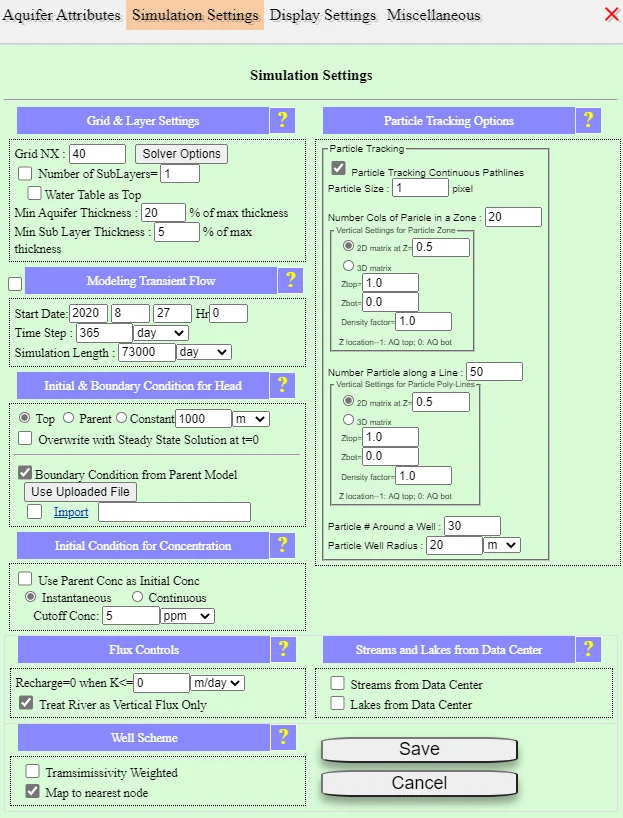
of nodes in the x- (west-east) direction, namely Grid NX. Here you can change the number from 40 to one that you prefer. The number of grid cells in the y- (north-south) direction is automatically calculated from NX and the shape of the model domain (e.g., if the model domain is longer in the y-direction than the xdirection, NY > NX). Achieving more accuracy, or resolving some groundwater system dynamics – for example, the quick changes in hydraulic head in the vicinity of a pumping well – require more model resolution (more nodes), so you will want to increase NX to, say, 80 or 100. (The maximum number of grid cells in X direction for the student version of MAGNWT is NX_max = 150. The total number of grid cells in both the X and Y directions for the student version of IGW-NET is NYNY_max = 100 * 100 = 10000.) However, it is good practice to use the default number of grid cells (NX=40) to understand the big picture and experiment with different aquifer representations before increasing the number of grid cells. An alternative to increasing the number of cells in the model is to make use of nested submodel, which can be interactively added and simulated in different, smaller areas of interest. This useful approach is discussed in the next subsection.
5.2 Defining a Nested Model
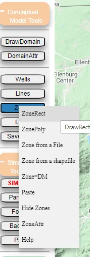
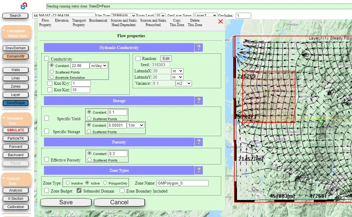
The model that we have defined above is called a basic "parent" model. By default, the boundary conditions on these models are assumed to be no flow and the model results are often not very accurate near the boundaries. However, knowing that the parent model is more accurate away from the boundaries, we can use smaller, nested “child” models to get more details (model resolution) in the areas of interest, using the flow information from the parent model to assign boundary conditions to the child model. The procedure to do this is presented in this Section. Begin by going to Zones and then Zone as shown in Figure 29. Then construct a rectangular area such as shown in Figure 30. The ZoneRect drawing tool functions like the DomainRect tool discussed in Section 3, i.e., you use mouse clicks to define the shape and size of the rectangle. Click ‘SaveShape’ to finalize the geometry; this action automatically launches the Zone Attributes menu shown in Figure 30. (NOTE: the submodel boundary is this example is relatively close to the left (western) boundary of the parent model, which we typically try to avoid; however, in this case, the western boundary corresponds with a large surface water body that is a dominant surface seep, making the model more accurate than in the case of no surface water body corresponding with the boundary). In the default tab (Flow Property), there is a box next to “Submodel Domain” under the Zone Types subsection. Check this box and click ‘Save’ to tell IGW-NET to use the zone as the simulation domain. However, before the zone will be recognized as the simulation domain, an important distinction must be made in the Domain Attributes menu: go to Conceptual Model, then Domain Attributes, then access the Simulation Settings and put a check mark in the box adjacent to Boundary Condition from Parent Model (Figure 31). To proceed with the nested submodel simulation, click SIMULATE. (NOTE: It is also possible draw an entirely new model domain using the DrawDomain tools but still use parent model results to assign boundary conditions in the new, smaller model, but the parent model will be “lost”. Using a zone feature to represent a nested submodel allows the user to retain the regional model domain). A series of three windows are presented in succession as shown below as Figs.Figure 33, Figure 34, and Figure 35, and you click OK to each. By clicking on the last of the three, the simulation begins. The submodel solution is presented in Figure 36. If the no-flow boundaries imposed on the “parent” model were active in the “nested” model, the contours would be orthogonal to the boundaries of the “nested”
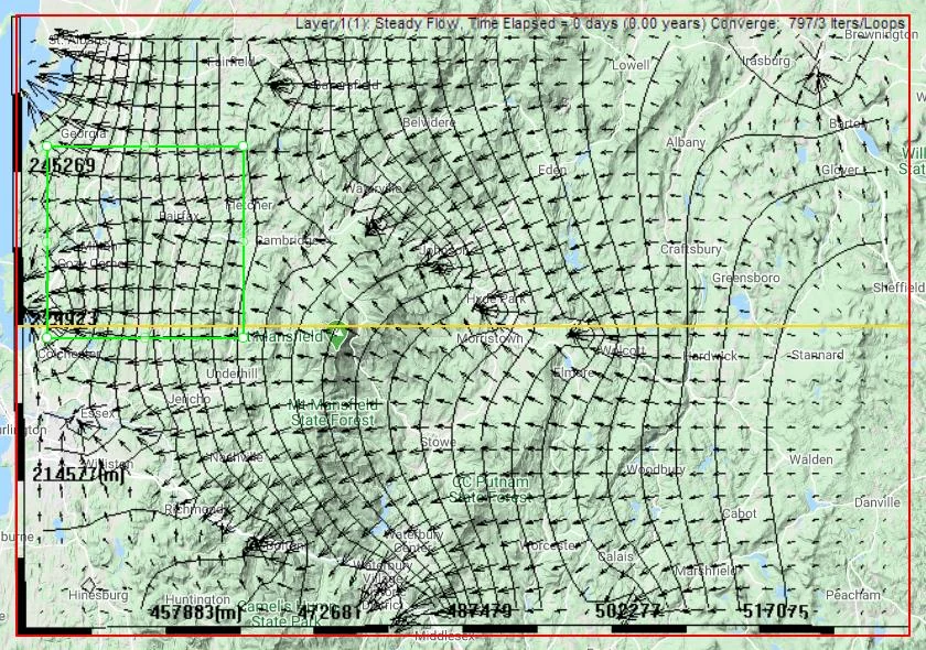
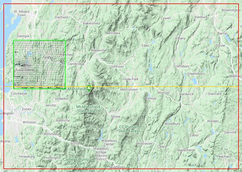
model. But they are not because the nested model uses constant head boundaries derived from the “parent model”.
5.3 Adding Surface-water Bodies as Conceptual Features
Earlier in Section 3.2., we learned how IGW-NET treats the land surface as a drain to account for the aquifer drainage effects of lakes, rivers/streams, and wetlands/springs. But we may want to treat the lakes differently, for example: as a source of water to the aquifer. An instance where this would be needed is when a pumping well is withdrawing groundwater near a stream, inducing water to move from the stream, into the aquifer system, and ultimately discharging to the well.
We now are going to add surface water bodies as conceptual features in our submodel, which will come in two flavors: lakes and similar quiescent bodies of water, and rivers and streams. We discuss them individually.
5.3.1 Adding a Two-Way Lake
To add a surface water body that has significant areal extent, that is, it cannot be approximated using a single line, it is necessary to define the location and geometry of this surface-water body. To do this click on Conceptual Model Tools and then on Zones. Several options will be available (see Figure 37).
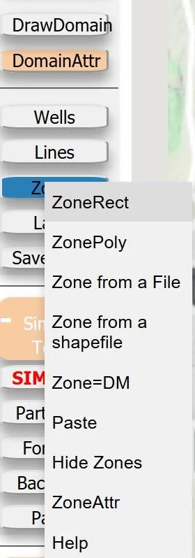
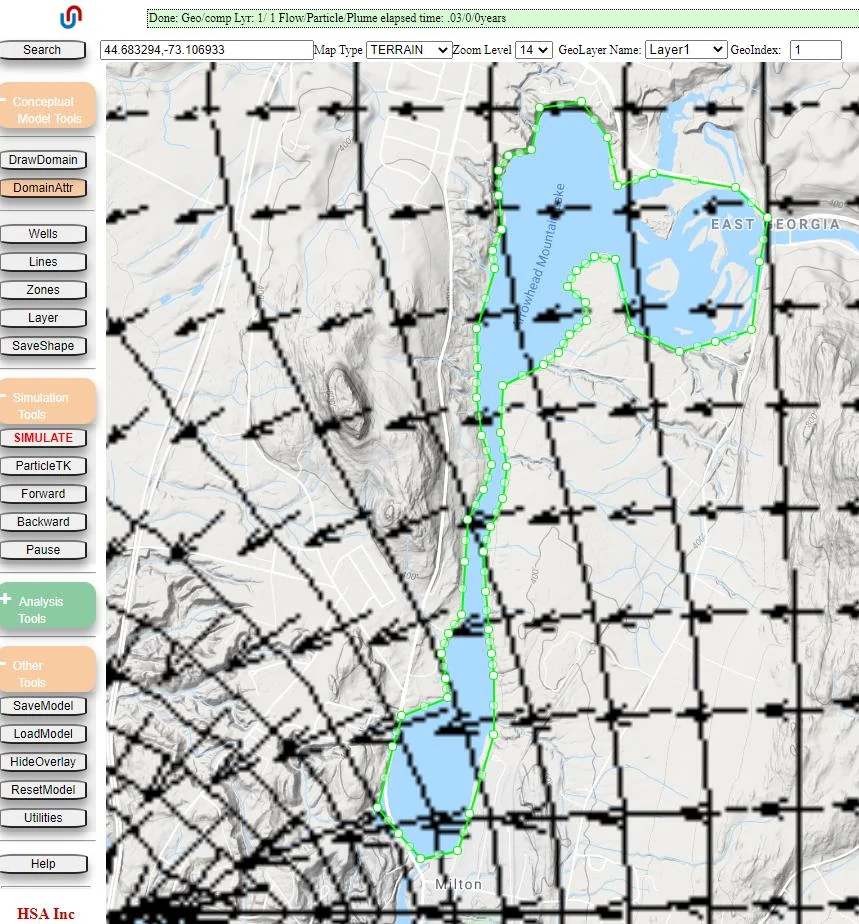
Now click on ZonePoly. This will provide you with a plus sign as a cursor with which you can draw a polygon. To draw the polygon, you click on a point on the model that is on the border of the area you wish to designate as the surface water body. Next move a small distance along the perimeter of the surface water body and click again. You have now created a polygon with two points. Not very interesting! Continue to move around the surface water body in small increments, clicking at the end of each increment, until you
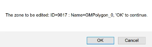
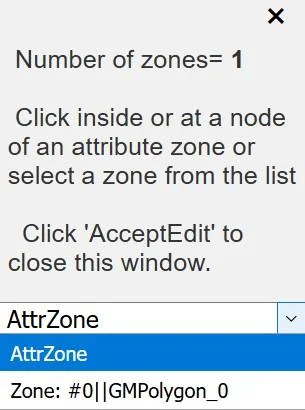
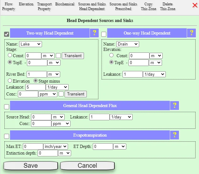
return to the location at which you started. Click once again on the first point you generated. You have completed the polygon. An example is shown in Figure 38. The area within the polygon is your lake. To give the lake descriptive parameters, click ‘SaveShape’; alternatively, you can: return to Conceptual Model and then click Zone, and click on Zone Attr to access the parameter input page. The drop down menu (Figure 39) reveals that we have only one zone, so we click on that. This spawns a the following message (Figure 40) to which we respond OK. Along the top of the window there are several options. This is because this ribbon is used to provide input for six different situations. Each choice can be used to define properties within your polygon. So, for example, if you wanted to define a different hydraulic conductivity over a specific region than what occurs elsewhere in the model, you could draw a polygon to define the area where you want the different hydraulic conductivity and then enter the value for that region. It will replace the one originally assigned in that region with your value. However, we are interested in the properties of the lake we have defined. To make changes to the lake we click Sources and Sinks Head Dependent (Figure 41). In the upper left-hand corner of this figure we see the notation Two-way Head Dependent. This is the panel we need, but what it means requires a little explanation. We need to be able to have water either enter or leave the lake depending upon the relative elevation of the hydraulic head below the lake and the elevation of the lake surface. For example, if there is a period of drought when the lake level is low so there is a hydraulic head in the aquifer below the lake that is higher than the water level in the lake, we need to have water move from the groundwater system to the lake. In other words, at the interface between the stream bottom and the aquifer there would be a negative gradient from the aquifer to the lake. On the other hand, if there is abundant rainfall and the river level is higher than that in the aquifer, we would expect water to flow from the river into the aquifer. This situation where water can either enter or leave is defined as a ‘Two-way Head Dependent’ condition because water can either enter or leave the lake depending upon hydrologic circumstances. Returning to the upper left-hand window we see that we have a Lake defined (window adjacent to Name). The stage is the elevation of the water level in the lake relative to a reference elevation. It can be specified as a number that is constant in time and space. If this is your choice you click the radio button next to Const and specify a value. It is often convenient to check the option TopE for the stage where TopE is the top elevation taken from the map (DEM). If you wanted to modify the choice from the DEM, you can replace the value in the box adjacent to the TopE notation with a suitable value. For example if you wanted to have the stage one meter lower than the elevation determined from the DEM, you would replace the zero with a one. Once the table is filled in, click the little white box to the left of the heading ‘Two-way Head’ and then click Save. One sees that there are two other options for how one treats the lake. These choices are variants on the one we have selected and their specific attributes can be determined by clicking the ? at the end of each descriptive title.
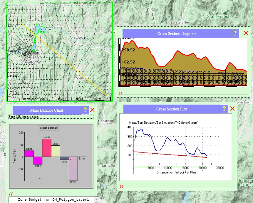
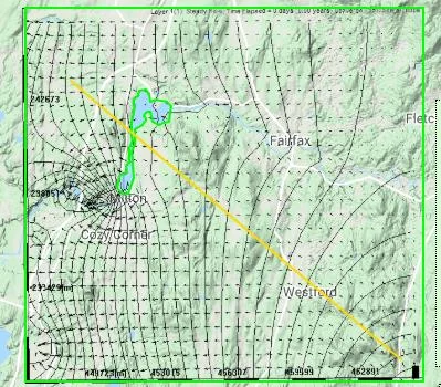
then click X-Section. After you have finished drawing the cross-section, go to Analysis Tools and click the Analysis button. From the list of options, click Display Charts. The new cross-section results will be shown in the Cross Section Diagram and Cross Section Plot charts (see Figure 45). Also note the updated water balance (amount of water moving into and out of the system) now includes Lake terms to represent flow to or from the lake (negative flux = groundwater lost to the lake; positive flux = lake water added to the aquifer).
5.3.2 Adding a Two-way Stream
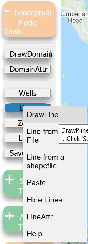
Let us now further extend our modeling capabilities to accommodate a stream or river. The major conceptual change is that we will now consider the surface water body to be a line rather than an area. To begin the process click Conceptual Model Tools, then Lines, then DrawLine as shown in Figure 46. Once you click DrawLine the large plus sign will appear on your model and you can trace the course of your river (in this case, we will trace the upstream portion of the Lamoille River). The trace of the river will be made up of connected dots as was the case with the lake boundary. Each click will produce a dot. The end result appears as in Figure 47. Now click on SaveShape. The Line Attributes window will open as seen in Figure 48. You have some choices here as to how you describe the hydrodynamics of the river aquifer system.
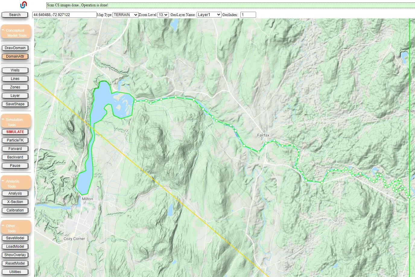
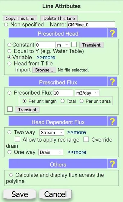
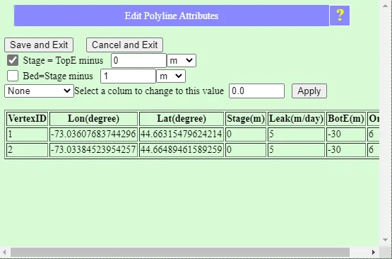
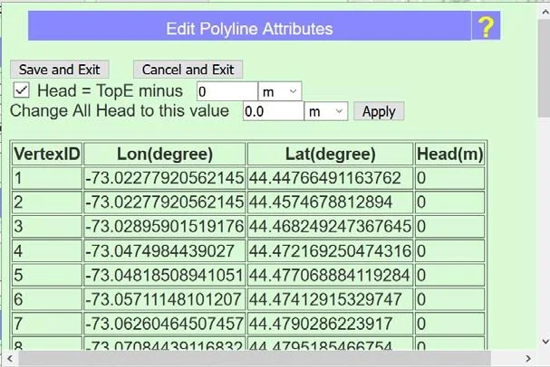
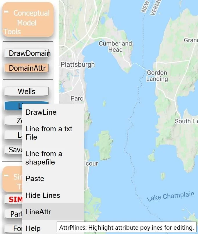
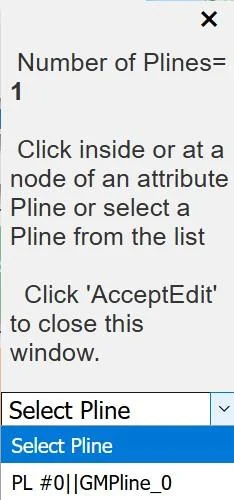
The simplest is to use the Prescribed Head option and a constant head value. To do this you click the radio button for Constant and replace the zero value with the river elevation (head) that you wish to assign. A variant on this is to allow for a variable river stage along the rivers course. To do this you click the radio button in front of Variable and then click ‘>>more’. This launches the menu shown in Figure 49. Here you can specify the river stage as the land surface elevation less a specified value. This allows for the provision of a river reach that has a sloping surface, which is the realistic option. The prescribed flux allows for the specification of leakage into and out of the stream directly. The head dependent flux option is similar to the treatment applied to the lake (see previous subsection), and it is the treatment we will use now. Choose the radio button next to Two way and then click the >>more button to open the Edit Polyline Attributes submenu (Figure 50). Again, you can specify the stage as the land surface elevation less a specified value. Use all defaults options and click ‘OK’ to close the menu (click the ? button to get complete details of this submenu). At the end of the input process click SAVE. You may decide to modify the attributes of your river or to draw another segment. The procedure for the case of changing river properties is presented in Figure 51. You begin by clicking on Conceptual Model Tools, than on Lines, then LineAttr. At this point you see the window presented as Figure 73. Note that the option of Line Attr is no longer available, but has changed to AcceptEdit. Let us repeat the process for the downstream segment Lamoille River: trace the river section using the DrawLine tool and treat it as a two-way head dependent boundary condition as described above. The resulting line feature is shown in Figure 53.
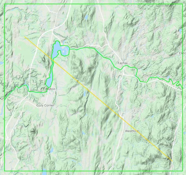
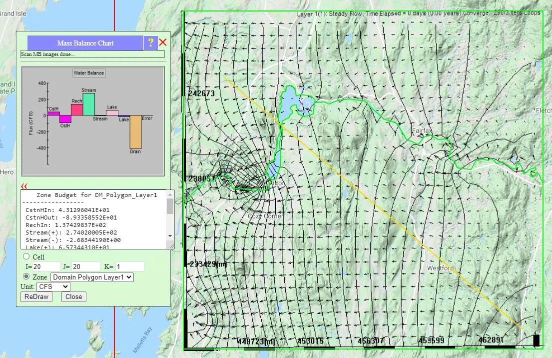
We are now ready to simulate our system and we go to Simulation Tools and then SIMULATE. Then we are greeted with the “projection system message”, and upon clicking OK yields the solution provided as Figure 54. Again, show the results in “chart view” by navigating to Analysis Tools, Analysis, then Display Charts. Figure 54 shows the flow field we have obtained using all the various conditions described to this point which now includes the river. Also note that new ‘Stream’ terms were added to the aquifer water balance. Apparently, under this model representation and grid resolution, the Lamoille River is serving primarily as a source of water to the aquifer, although in some areas groundwater is clearly converging to the river.
5.4 Adding Wells
Let us now look at the impact of introducing a pumping or injection well into the simulation. This requires modeling with higher resolution (more details), which can be done by modeling a smaller area, or by increasing the number of grid cells of the simulation “mesh” as was explained in Section 5.1. We will adjust the size and location of the zone being used to define the submodel domain. Go to Other Tools, then Utilities, then Geometry unlocked’ to show the vertices (nodes) of the submodel zone (it may not be necessary if the zone is already unlocked). Click-drag on any of the nodes to adjust the submodel domain to cover the small populated area south of the lake (see Figure 55). We will add a water supply well (pumping well) near the center of model. To add a well to the model you click Conceptual Model Tools and then Wells. The following window will appear (Figure 56). Now click Draw Wells. A plus sign will appear that you can move with your mouse. Move the plus sign to the location where you wish to locate a well and click your mouse. The following
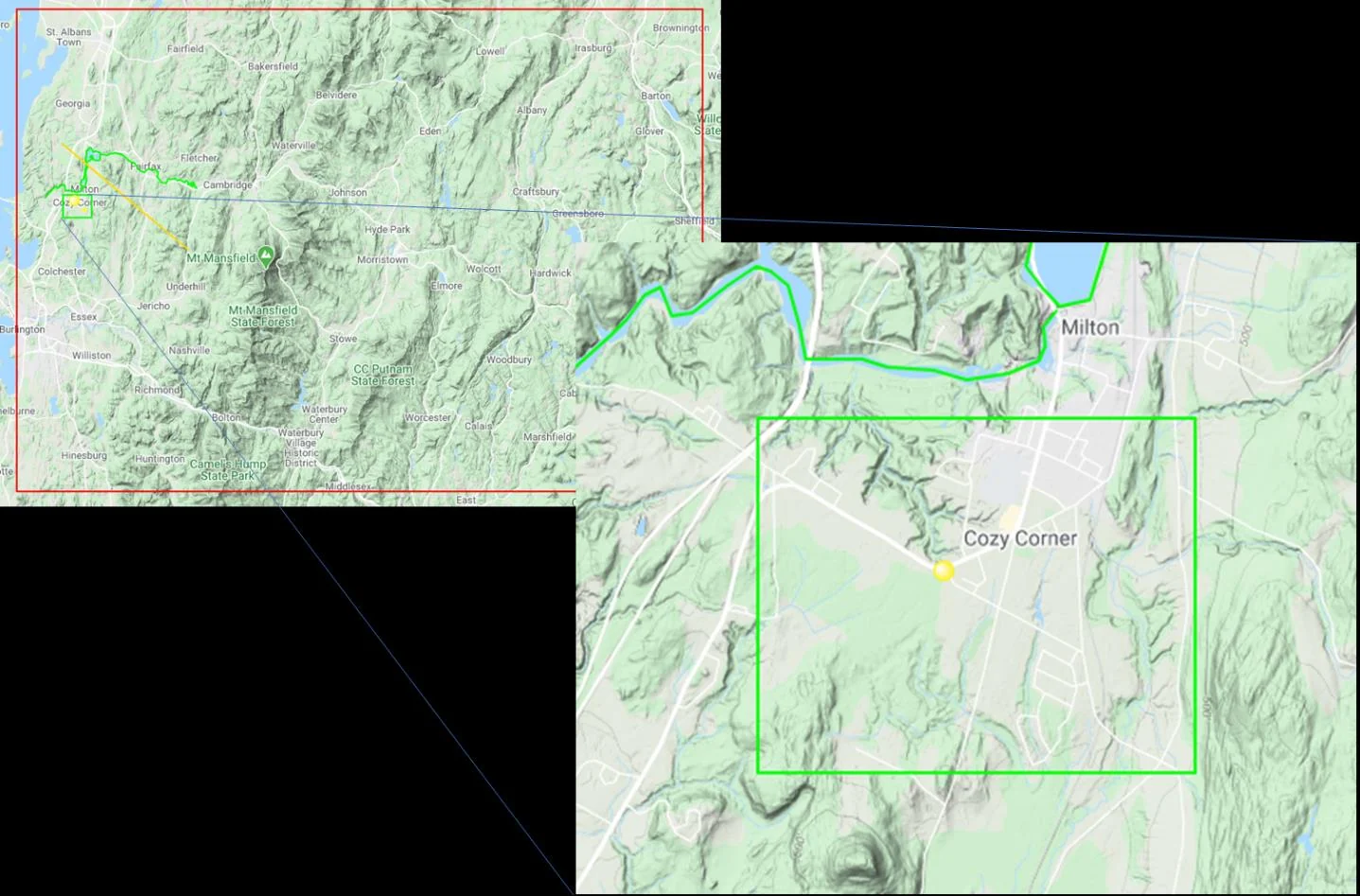
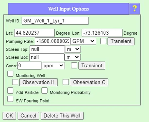
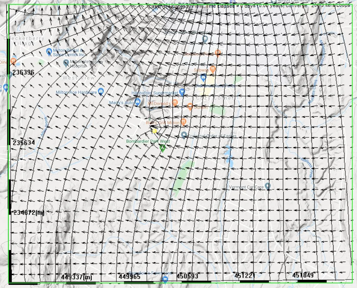
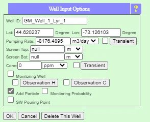
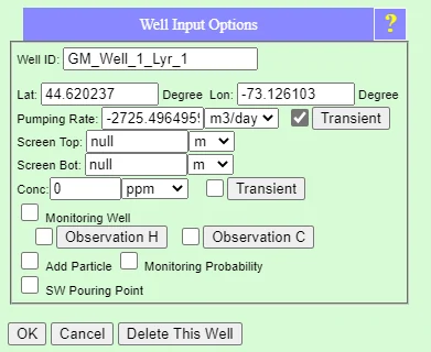
window will appear (Figure 57). The inset window is the information pertinent to the well you just located. You can now change the pumping rate from 0 to the value appropriate for this well in your model. There are several options but the one that you may need later is the specification of a particle. Later we will be using tracer particles to establish where groundwater flow in the model. Note that this is also where you can delete a well. You are now ready to simulate the impact of a well in the area you have selected for your model. The same process you used earlier to simulate the behavior of the hydraulic head is repeated. If you click on SIMULATE under Simulation Tools you will see prompts regarding resetting the model and the model projection (accept to proceed). The resulting flow field is shown in Figure 58. One can see the local convergence of groundwater and a head depression near the well in response to the pumping. If you examine the water balance, you will see that the well discharge is small compared to the other sources and sinks of water (recharge, flow in/out of the model boundary, and surface seepage).
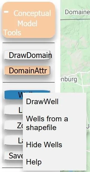
5.4.1 Delineating a Wellhead Protection Area (Source Water Area)
When a well is used for drinking water supply (or even irrigation water), it is often necessary to delineate a wellhead protection area, or the source water area contributing to the well, so that potential sources of contamination up-gradient from the well can be identified and mitigated/eliminated. In IGW-NET, we can delineate a wellhead protection area by adding particles to a well and trace backwards from the well the flow pathlines. In section 4.2, we learned how to add particles along a line drawn in the model domain. The process for adding particles to wells is much easier. Simply click on the well marker (yellow “pushpin”) to open the Well Inputs Options menu. Find the box next to Add Particle and check it (see Figure 59). Then click OK. Particles will be placed around the well at the onset of the next simulation
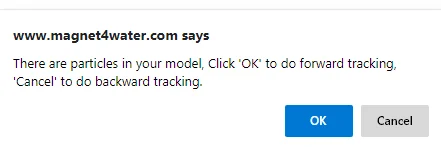
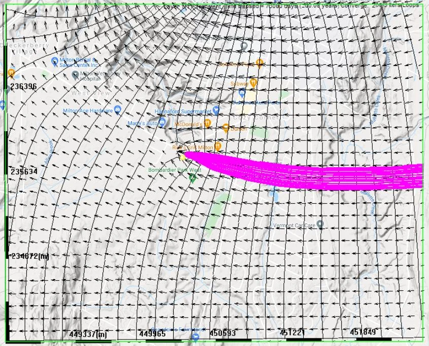
Click SIMULATE and proceed through (click OK) the familiar prompts regarding resetting the model, obtaining boundary conditions from the parent model, and using the identified projection system. Then you will see the prompt regarding forward versus backward tracking that we saw before (shown again in Figure 60). Click cancel to perform backward particle tracking. When the groundwater model is finished running, particles will begin emanating backward from the well along the solved flow field. The “envelope” of particle pathlines gives an estimate of the groundwater source water area for a given period of time. The particle envelope will continue extending back along the flow field until the simulation period is over or the particles reach a boundary (see Figure 61). We will next explore how particles can be used to model transport of chemicals. Once the particle tracking is completed, open up the Well Input Options menu once again, and uncheck the Add Particle box to remove particles from the well location. Click OK.
§ 6 Modeling Transport
6.1 Estimating Potential Impact Areas with Forward Tracing Particles
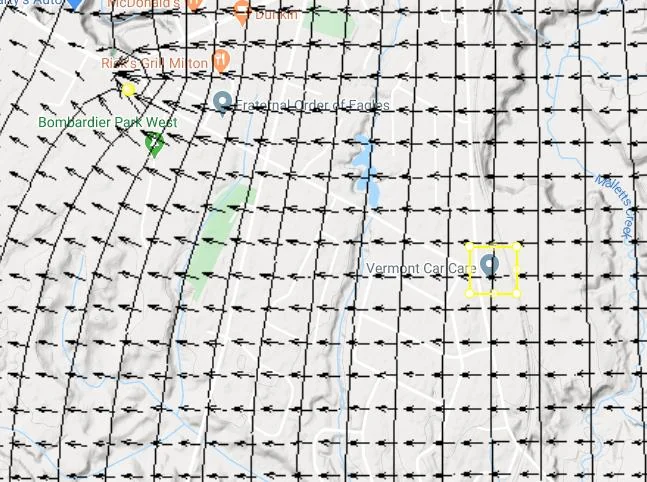
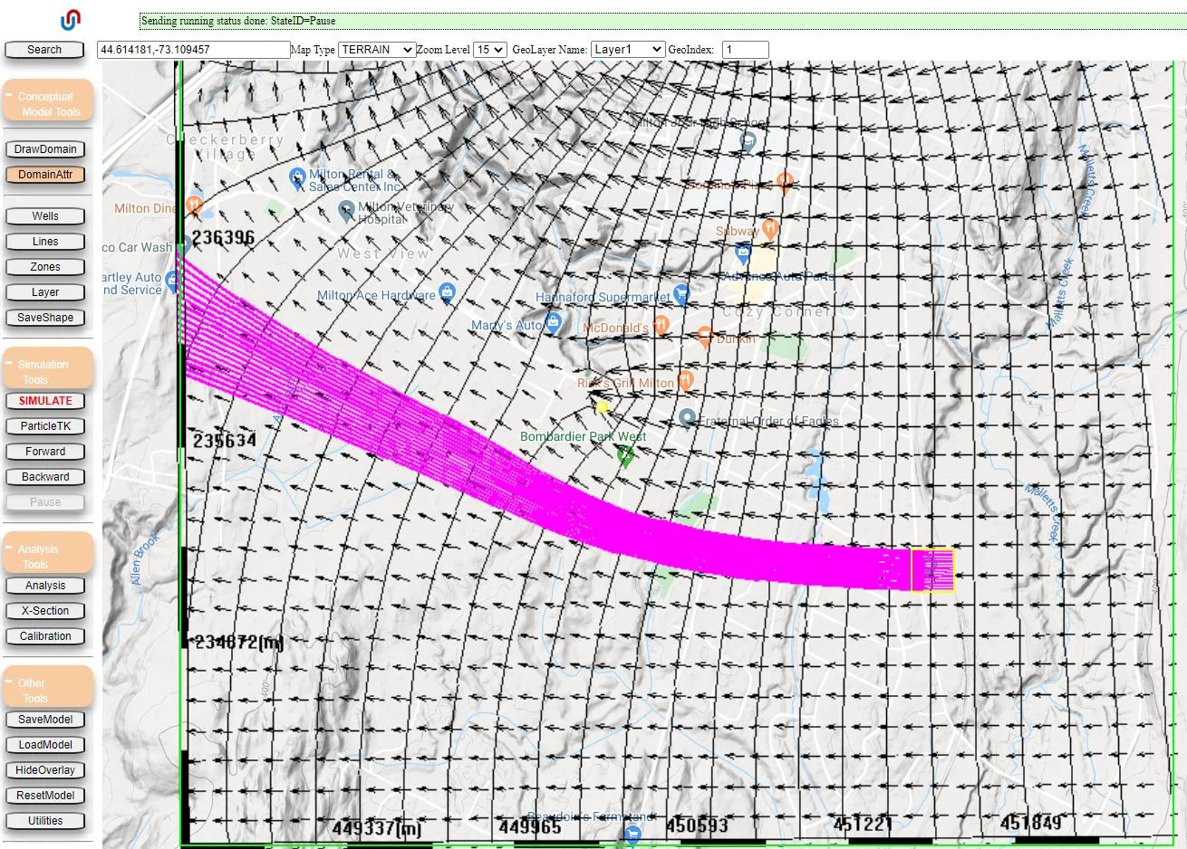
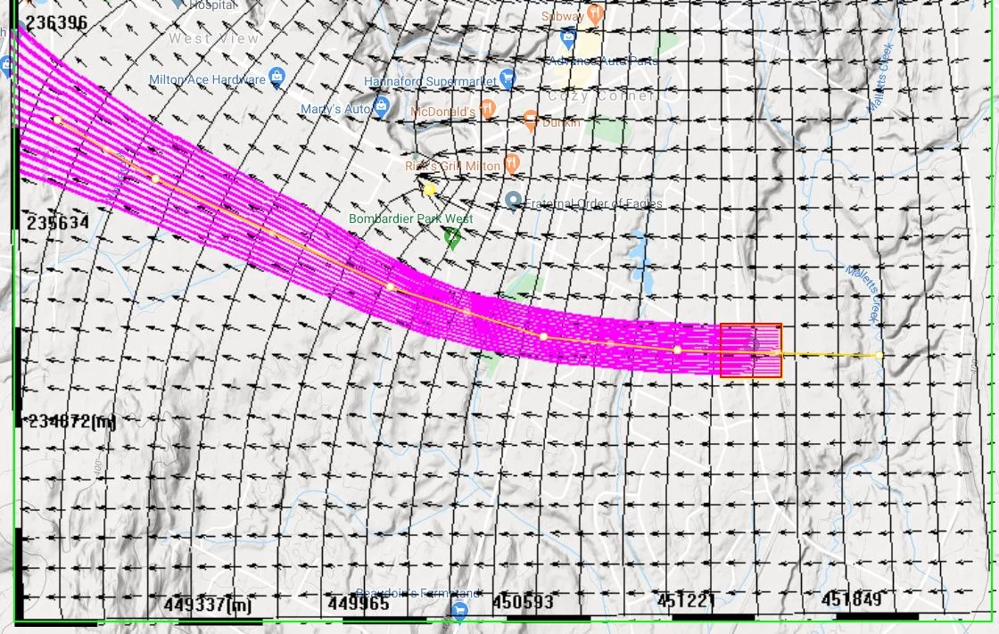
There are several factors that can affect movement of a contaminant. This includes mechanical dispersion and molecular diffusion, reactive decay of the chemical and sorption interactions with soils and sediments (partitioning). But one thing that is always important (and is often the dominant factor) is the movement of the contaminant due to the flow of groundwater – or advective transport. We learned early in Section 4 how to use particle tracking to visualize groundwater pathline, which is the trajectory that individual fluid particles follow in a steady-state flow field So, if you want to see where a contaminant has gone over a period of time, particle tracking is a useful tool. In Section 4.2.3, we learned how to access the Particle Tracking placement tools by going to Simulation Tools and clicking the ParticleTK button. Now, we will select the ParticleRect option so that we can place a particle rectangle at the location of a hypothetical source of contamination. Add a rectangle over the Vermont Car Care business (as a hypothetical source of groundwater contamination) in the same manner you would add a rectangular zone: use a single-click to indicate the position of one corner of the rectangle, and another to indicate the position of the corner that is diagonal from the first placed corner (see Figure 62). Click SIMULATE after the rectangle is added to re-submit the model for solving. The usual prompts regarding resetting the model and the model projection system will appear; but you will also see a prompt related to performing forward or backward tracking of the particles along the steady flow field 9see Figure 63). We wish to do forward tracking, i.e. determine where contaminants at the specified particle locations will go, so click OK. When the new model results appear, particles pathlines will begin emanating from the “contamination site” and will flow along the simulated flow field based on computed velocity vectors, over time tracing out the “envelope” of the potential area of impact downgradient from the site (see Figure 64).
6.2 Identifying Potential Sources with Backward Tracing of Particles
Particle tracking can also be useful for identifying potential sources of known groundwater contamination. The idea is to add particles at the location of interest, track the particles backward along the flow field, and compare the pathline envelope to possible surface or subsurface sources of contamination. The process for computing and visualizing particle pathlines is the same as described above: add particles using the ParticleTK button options, and click Simulate. But now select Cancel to the prompt regarding forward verses backward particle tracking so that IGW-NET applies backward tracking.
6.3 Predicting Chemical Concentrations
We will now use IGW-NET’s transport analysis tools to simulate the concentration distribution of dissolved species (chemicals) originating at the hypothetical site used in Section.
6.2.1 Assigning Sources
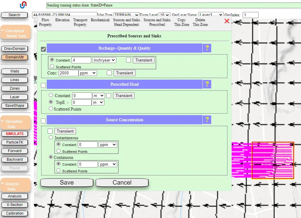
A chemical source can be assigned in a number of ways, for example: as a zone representing a continuous source or a instantaneous source (all mass added “at once”); from an injection well, from a headdependent source/sink (e.g., a polluted lake or drain), from the surface with a prescribed rate of infiltration (recharge). We will add a zone feature and assign it as a surface source with an infiltration rate of 4 inch/year and a source concentration of 2000 ppm. To do this, we go to Conceptual Models, then Zones, and then click the ZoneRec. Draw a rectangular zone in the same location as the particle zone that was used in the last simulation. Click ‘SaveShape’ to open the Zone Attributes menu for the newly added zone, and navigate to the Sources and Sinks Prescribed tab (see Figure 66). Check the box next to ‘Recharge – Quantity and Quality’, and enter a value of 4 in the text field next to ‘Constant’. This is the prescribed rate of infiltration (units: inch/year). In the text field next to ‘Conc’, enter a value of 2000 (units: ppm). This is the source concentration. Note that it does not change with time, although it is possible to make the source concentration vary with time, or the contaminant can be released at once as an ‘impulse’.
6.2.2 Assigning Dispersive Properties
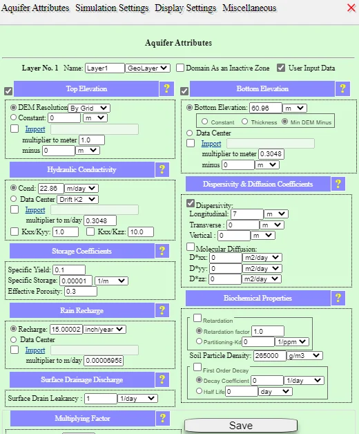
As we discussed earlier, transport of a contaminant is controlled by advection, but also is impacted by mechanical dispersion and/or molecular diffusion. In some cases, biogeochemical processes might be important, for example, reactive decay or sorption to soils and other solids. In IGW-NET, you can assign dispersity and diffusion coefficients or biogeochemical properties within the Aquifer Attributes tab of the Domain Attributes menu (Conceptual Model Tools, then DomainAttr). (Note: you can also specify these parameters using zone features, but the applied properties only apply with that zone.) We will assign longitudinal (i.e., along the pathline of the fluid flow) dispersivity coefficient of 7m in this example (see Figure 65 (longitudinal dispersivity coefficient typically can vary from 5 to 100m). Dispersion acts to dilute solutes its groundwater and lower their concentrations and is a result of mixing of contaminated fluid with uncontaminated fluid in the porous media.
Click Save to close the Domain Attributes menu and preserve the changes.
6.2.3 Simulating and Visualizing Transport
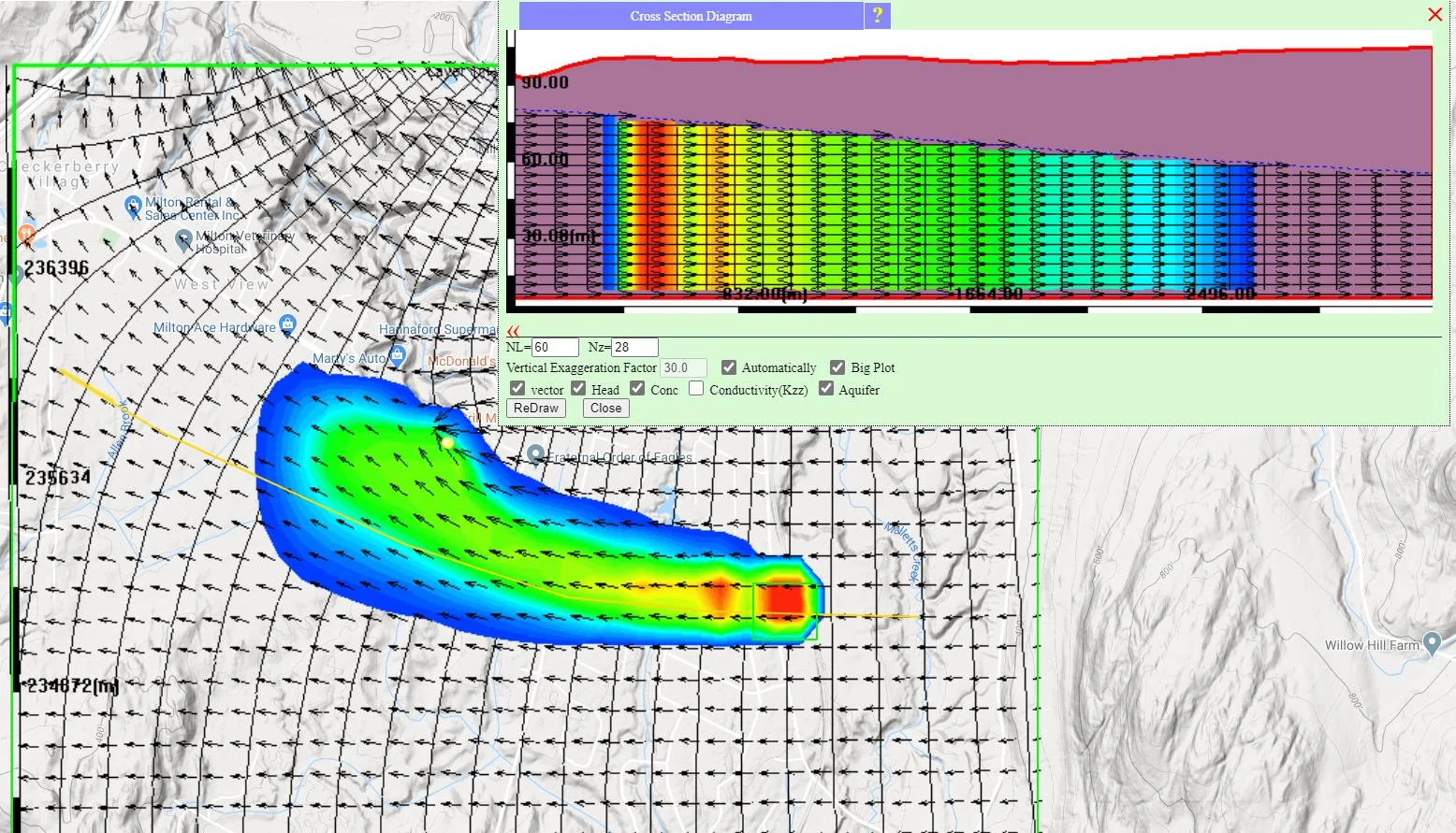
Next, we want to delete the particle zone now that we have added a chemical source. To do this, click on Simulation Tools, then click Particles, then click DeleteParticle. This removes any particle features included in the model domain, including the particle rectangle. Note that the pathlines will not be removed until a new simulation is returned to the map display. We will want to visualize the plume in both plan view and cross-section view when we re-submit for simulation. Use the X-section tool under Analysis Tools to draw a new cross-section through the center of the “potential impact area” determined from particle tracking (see Figure 67). Now we are ready to submit the model for flow and transport simulation (click SIMULATE). Again, the flow field is steady (does not change with time), but the contamination plume will evolve over the course of the simulation and the results are shown in the map display Figure 68. We can see significant spreading of the plume, caused by the use applying longitudinal dispersion and by the relatively coarse grid size (NX=40) that causes “numerical dispersion” or artificial spreading when numerically solving the transport equations. The cross-section diagram (accessed under Analysis Tools, Analysis, then Display Charts) shows a plume that is vertically-mixed, as we expect given that we are simulated 2D groundwater flow in this example (i.e., no resolution of vertical details). In the next section, we will learn how to resolve vertical details by adding more layers to the model.
§ 7 Adding Vertical Layers to the Model
While a two dimensional model such as we used earlier is typical of those used in most applications, the use of such a model implies that the geological materials do not vary significantly with depth and that there is not a significant vertical gradient in the hydraulic head. We also saw the need to resolve vertical details of contaminant transport which cannot be done with a 2D model. When we need more vertical details, it is necessary to add layers to the model. Think of each layer as a layer of a layer cake. Up until now we have had just one layer for our layer cake. Multiple layers can be used to represent the vertical components of the hydraulic head or to more faithfully represent a vertically varying or layered geology. There are two types of layers in IGW-NET: computational layers and geological layers. Computational layers are used to sub-divide a single geological unit into more than one “grid layer”. Geological layers are used to differentiate units with substantially different geologic characteristics (e.g., aquifer vs. aquitard). One way to think about the difference between computational layers and geological layers is to imagine a Rubix cube with the following characteristics. Imagine the Rubix cube is made from six square layers stacked on upon the other, each containing 36 small cubes. In total we have 6×6×6 = 216 little cubes.
Now further imagine that the first and second layers are red, the middle two layers are blue and the bottom two layers are yellow. In IGW-NET the three sets of colored layers, each having a thickness of two layers of the same color, would represent geological materials, perhaps the red could be sand, the blue clay and the yellow gravel. In this scenario each geologic layer would be represented by two layers of 36 small cubes. Now consider the six layers, independent of their color. These six layers are the computational layers and exist only to allow for a more accurate representation of flow behavior in the vertical direction. The more layers, the more accuracy in the simulated results, but the more computational work that is required to solve the system of equations. For example, in the one layer case we would have 72 equations to solve and in the six layer case 216 equations.
7.1 Adding Computational Layers
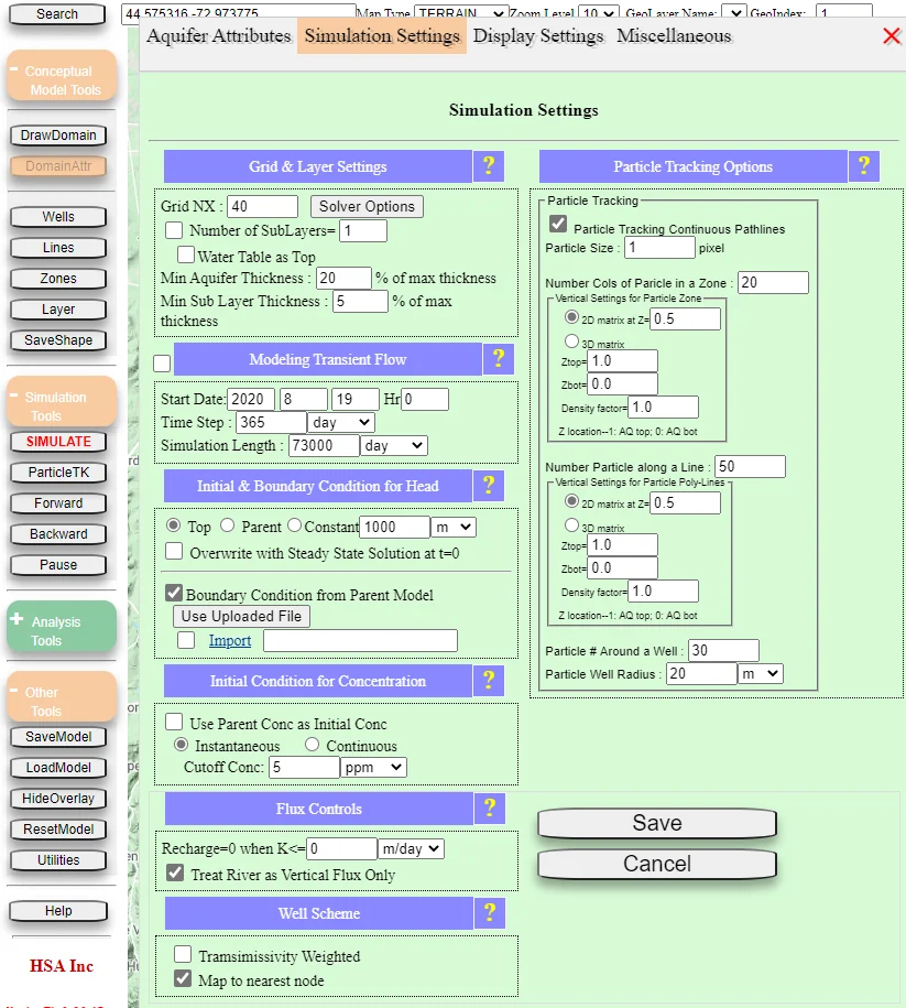
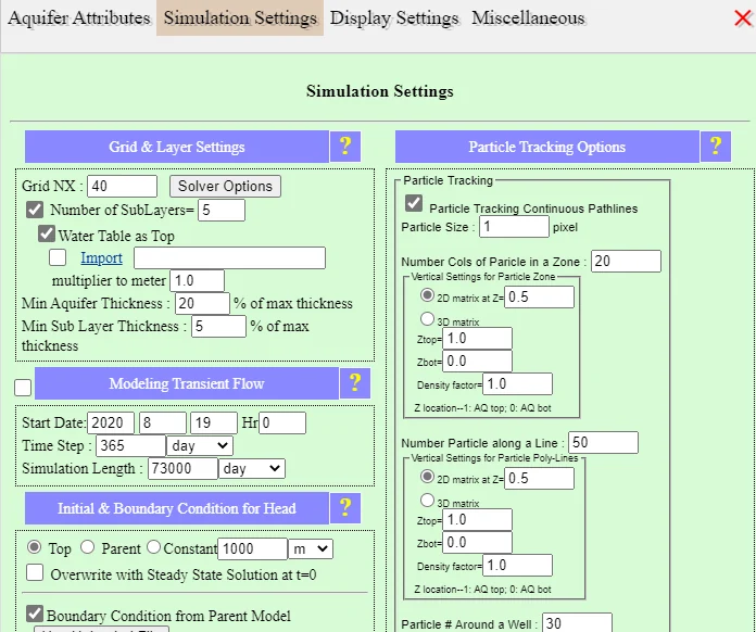
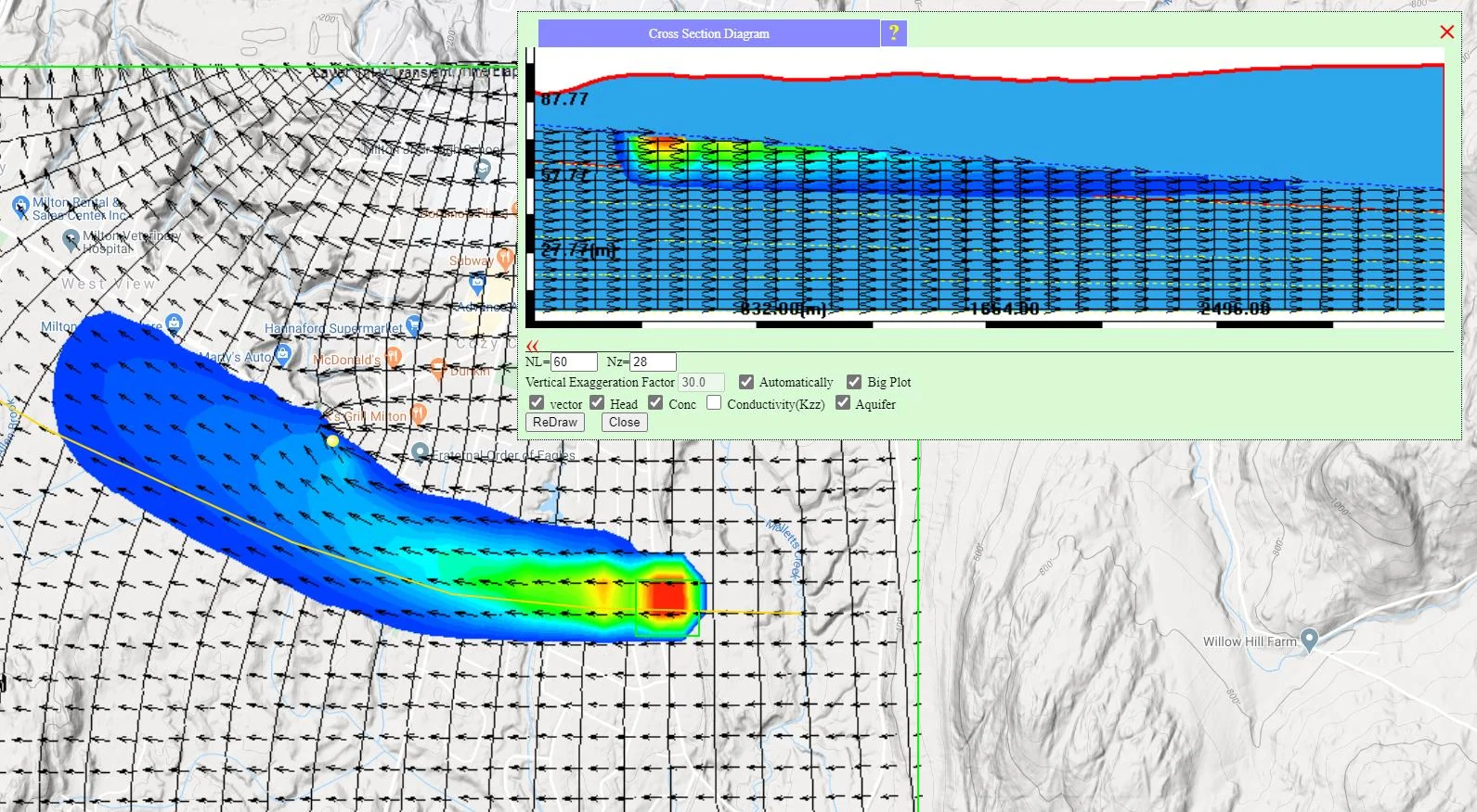
Now, to access the multiple layers option (that is, the ability to define the number of computational layers for a given geological layer), click on the Simulation Tools tab, then the Simulation Settings tab at the top of the screen. This then reveals the Simulation Settings window shown in Figure 69. Now click the box to the left of Number of SubLayers and put in the box to the right of Number of Sublayers the number of layers of interest. You should also check the box next to ‘Water Table as Top’. This tells IGW-NET to subdivide the aquifer following the simulated water table of your last model submitted to the IGW-NET server (you can also upload a saved model result). It is good practice to first simulate the 2D water table, then add computational layers and sub-divide following the 2D water table. Click SIMULATE to solve the new model with multiple computational layers. When you view the results in the cross-section diagram, you will see that the chemical source is being now added to the top of the aquifer or 1st computational layer (see Figure 70). You will also see the different computational layers as yellow dotted lines.
7.2 Adding a Geologic Layer
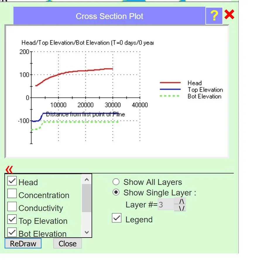
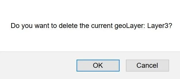
As noted, we have two kinds of layers and each has its own protocol for being added to the model. We will now add a geologic layer to the default condition of only one layer. To add a geologic layer we go to Conceptual Model tools, then Layers, and then Add a New Layer. Clicking Add a New Layer adds the layer we are seeking. It is added to the bottom of the model and has the same spatial extent as the top layer of the model. However, this layer can have a unique set of physical attributes such as hydraulic conductivity. Note that, if you make geometric changes to the top layer, such as its geometry, all layers below it are appropriately adjusted. Figure 71 shows the modeling environment after you have added a layer to the model. Clicking on the ‘v’ to the right of the word Layer in the Geolayer Name box reveals all the currently existing layers and if you click one of the other layers the information on the screen relates to that layer. You can delete any layer by going to Conceptual Model Tools, then Layer, then click Delete Current Layer. You can add a third layer (Layer 3) and then delete it using this approach (see Figure 72).
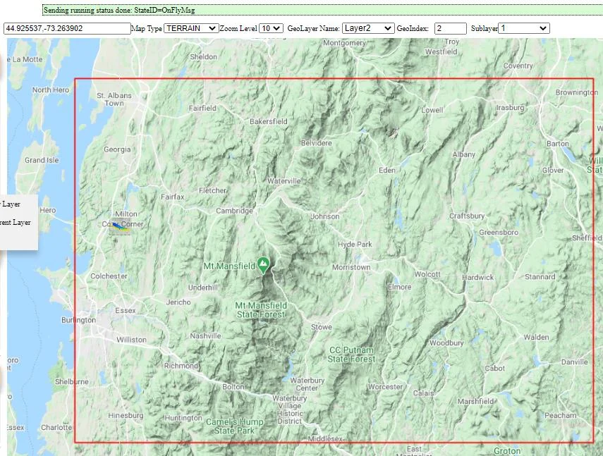
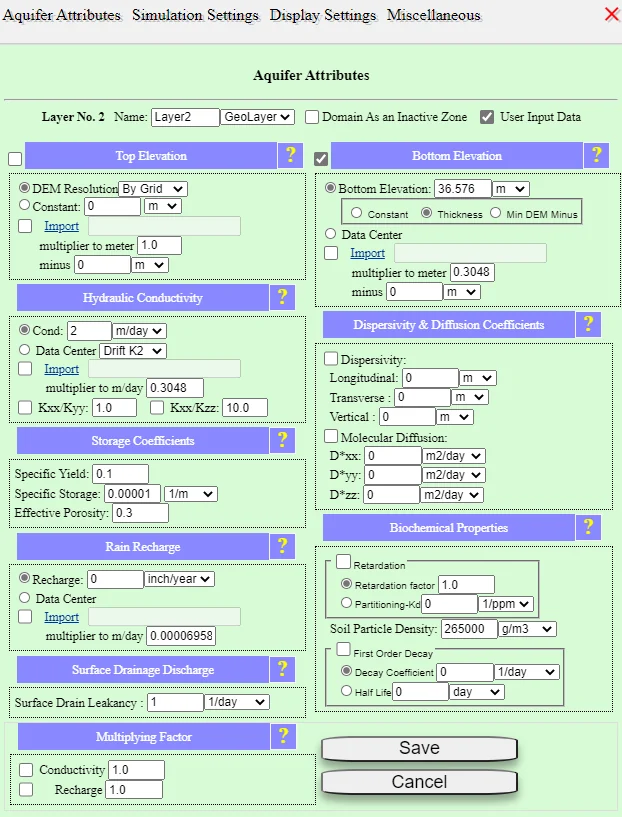
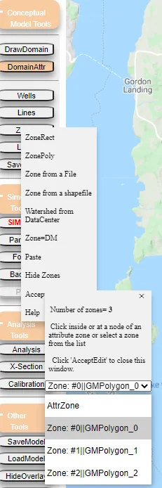
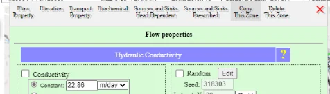
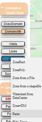
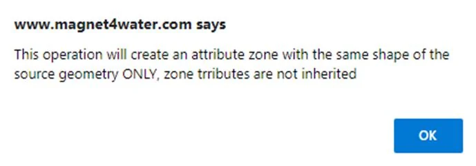
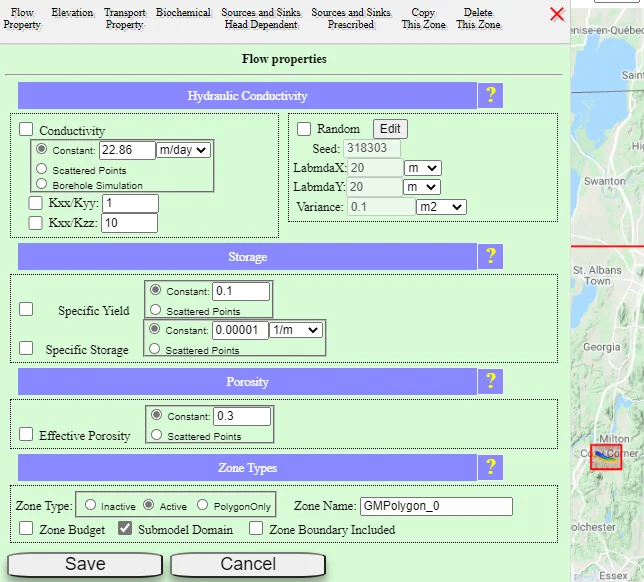
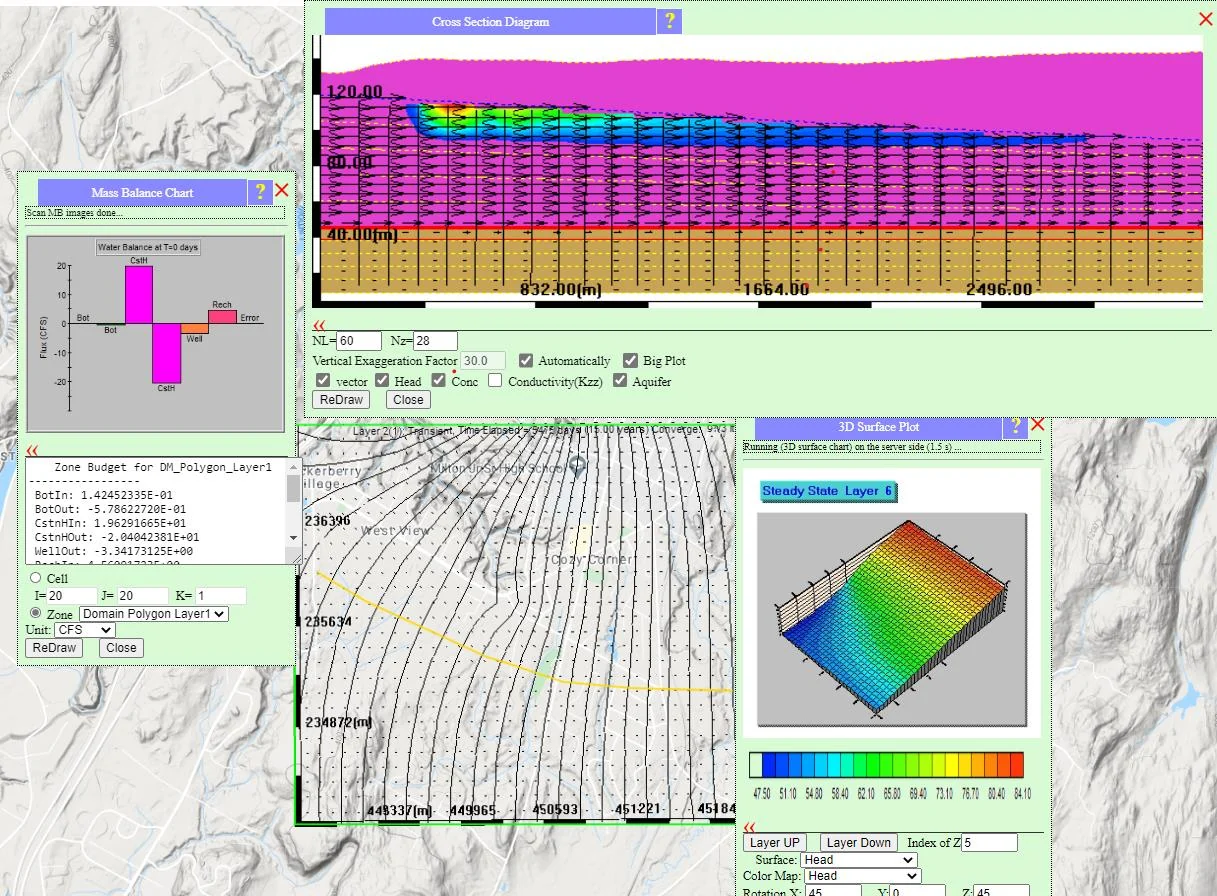
We now need to set the attributes for Layer 2. Change to Layer 2 using the drop-down menu mentioned above, and then click Conceptual Model Tools, then DomainAttr. This opens the Domain Attributes menu for Layer 2 (see Figure 73). Reduce the hydraulic to 2 m/day and see the aquifer thickness to be 10m (33ft). Note that you can navigate between layers from within the Domain Attributes menu (Aquifer Attributes tab) by using the drop-down menu called GeoLayer near the top. We next need to add the submodel zone to both layers to be able to properly simulate the 2-layer submodel. This is done by “copying and pasting” the zone from Layer 1 to Layer 2. Begin by navigating to Layer 1 and then accessing the Zone Attributes menu. You can access this menu through the ZoneAttr button (Conceptual Model Tools, then Zones, then ZoneAttr - Figure 74 ), as we discussed in section 5.3. Or, you can go to Utilities, then Unlock Geometry, and then click inside of the submodel zone in the map display. Once you access the Zone Attributes menu for the submodel zone, find the ‘Copy this Zone’ option along the top menu ribbon/tabs. Click it to tell IGW-NET to copy the zone to the IGW-NET “memory” (or clipboard) (see Figure 75). Now change to the 2nd layer of your model so you can “paste” the zone feature. To do this, click Conceptual Model Tools, then Zones, then Paste (see Figure 76). A prompt will appear telling you that only the geometry will be copied (no attributes) - click OK (Figure 77). The Zone Attributes menu will appear for the new zone added to the 2 nd Layer (Figure 78); make sure to check the box next to ‘Submodel Domain’ and then click Save. Click SIMULATE to solve the new, 2-layer groundwater flow and transport model, clicking through the usual set of prompts so that the simulation moves forward. We can view the plan-view results in each layer by switching back and forth using the drop-down menu at the top of the mapping/modeling environment. If we view the results in cross-section view, we can clearly see a 2nd layer add to the model and the difference in groundwater velocities between the two layers (see Figure 79).
§ 8 Modeling Unsteady Flow
To this point we have assumed that our flow model is time-independent. (NOTE: while we have modeling the evolution of particles paths or dissolved species distributions, the flow field was steady, i.e., not changing with time.) In this Section we introduce the concept of transient groundwater flow behavior. In other words, we will not assume the system is at steady state, but rather allow it to evolve through time from one state to another. To do this requires we define a new physical parameter that accommodates the elasticity of the aquifer (see Section 3.2).
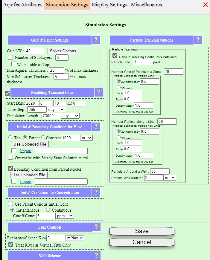
To indicate that we are performing a transient analysis we open the Default Parameters and Options menu. To get there you click Conceptual Model Tools, then Domain Attributes. Note that in the bar at the top of this window there is a Simulations Settings option that you must activate by clicking it. This action will yield the window shown in Figure 80. In the middle column, about half-way down the page, there is a Modeling Transient Flow option and to the left of this heading there is a small box that needs to be checked for transient flow to occur. Note that you should NOT enable this feature when performing particle tracking / contaminant transport on a steady flow field. You may still adjust the time-step for particle tracking / transport if the "box" next to Modeling Transient Flow is unchecked.
8.1 Simulation Time Settings
In the Modeling Transient Flow section of the Simulation Settings menu, you will see fields for inputting the simulation start date and time (hour of the day), the simulation time-step, and the simulation length.
You can use theses texts boxes next to ‘State Date’ (year, month, day), ‘Hr’ (hours), ‘Time Step:’ (days), and ‘Simulation Length’ (days) to define user inputs, but for this example we will use the default inputs. Note that the maximum number of time steps for the student version is 300. If you increase the simulation length, you will need to increase the time-step to ensure that your simulation reaches the end. If you decrease the simulation length, you can consider reducing the time-step to get more temporal resolution.
8.2 Initial Condition
To simulate a transient problem you need initial conditions (in addition to the boundary conditions you normally need to provide for a steady-state model). Initial conditions are the conditions in the aquifer at the time from which you wish to simulate behavior into the future. In our example we will take the steadystate solution we have just generated as our initial conditions, so we select ‘Parent’ from the set of options under the Initial and Boundary Conditions for Head section of the Aquifer Attributes submenu (see Figure 80). You could also use the aquifer Top elevation as the initial condition (e.g., corresponding to the inundated or flooded conditions) or a constant elevation. Finally, if you did not just previously execute the steady-state model, you can tell IGW-NET to first solve the steady-state solution and then use that as the initial condition.
8.3 Time-Varying Stress
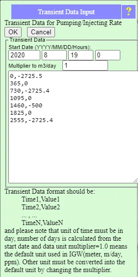
Since this is a steady-state solution we must change something in the system to make its behavior into the future different than what it has been in the past. The change we will make is introduce time-varying pumping rates to the well that we introduced in Section 5.4. To do this, click on the yellow pin/marker representing the well in the map display. In the Well Input Options menu that appears, check the box next to Transient next to pumping rate (see Figure 81). Then click the Transient button to open the Transient Data Input submenu for the well (see Figure 81). The starting date should correspond to the starting date set in the Simulation Settings described above. Then we can enter time-varying pumping rate data into the provided table, where each line is a (time, rate) data pair, where time is measured as the number of days since the starting date, and rate is the pumping rate in cubic meters per day (if you use different units for pumping rate, you can use the mulitpler to m 3/day text field to convert to m3/day). A pumping rate assigned at a particular day will be used until the pumping rate changes at a later specified time. When you are finished entering the pumping data, click OK to close the submenu, then click OK to close the Well Input Options menu.
8.4 Presentation of Transient Results
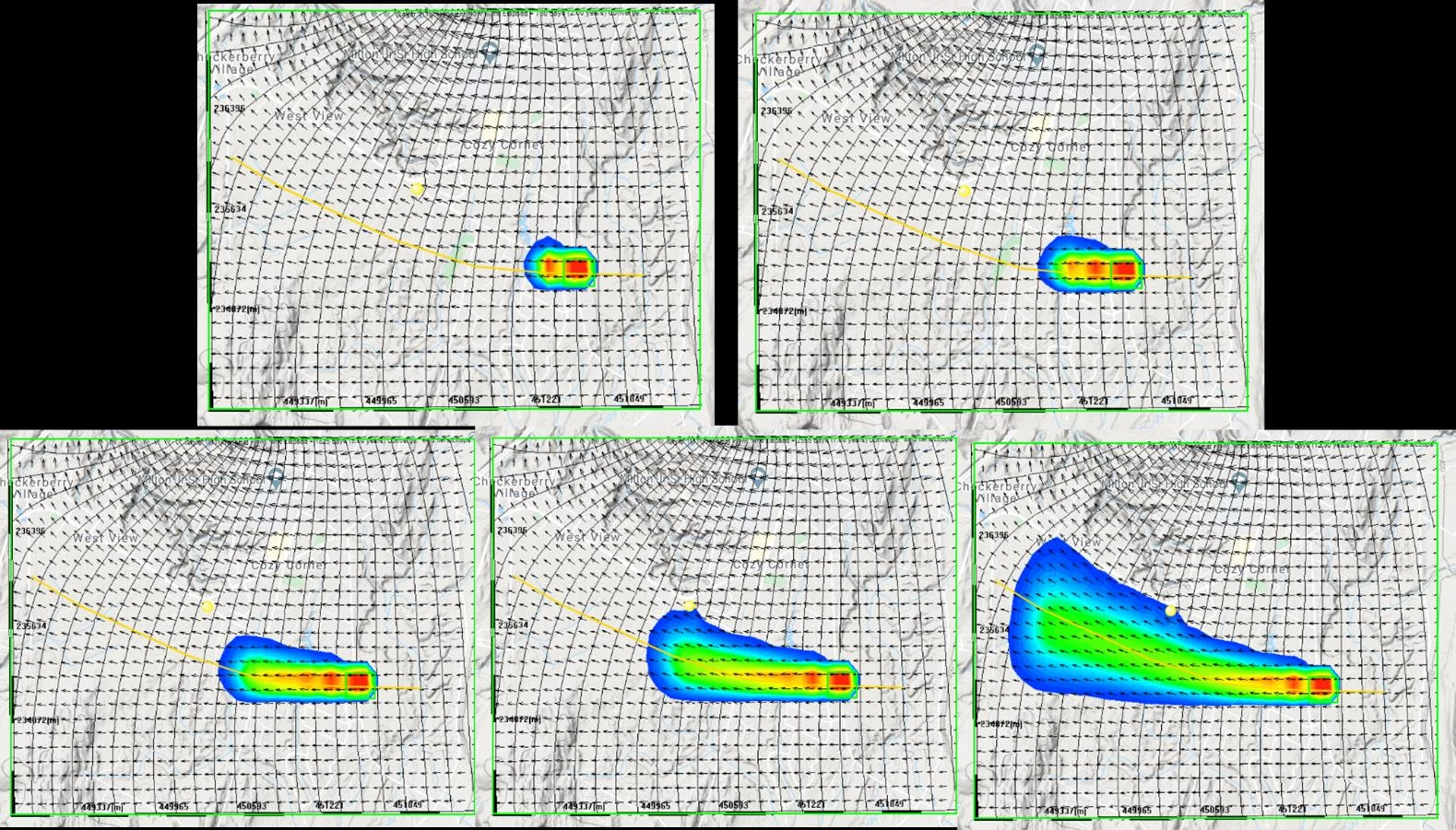
We are now ready to simulate in transient mode. Clicking on SIMULATE yields the familiar warning prompts; click OK and you will initiate the calculation. As the simulation is running, at the top of the plot you will see the elapsed simulated time (real elapsed time, not computer simulation time) and you can see the plot changing in response to the time-varying pumping rates (see Figure 83). Note how the contour lines around the well change in response to the time-varying pumping rates. In some cases, it might be difficult to notice the changes because the simulation takes place rather quickly on the computer so the results at different timesteps may pass quickly. In addition, the results may not change much over each time step, so the outputs for different time steps may seem pretty much the same. Just like steady-state simulations, it is possible to view the results in Chart view by clicking Analysis Tools, Analysis, then Display Charts. The familiar graphics will appear, but we will notice that some of the charts update as the simulation proceeds forward. For example, the mass balance chart will appear different at different time steps because of the time-varying pumping rates. If a monitoring well has been added to the model (see Section 5.4) a time-series head and/or concentration plot will be updated as the simulation proceeds. At any point, you can pause the simulation by clicking Pause under Simulation Tools. You can perform further analysis (e.g. draw a new cross-section), but when you are ready to proceed forward with the simulation, click Forward under Simulation Tools. In some instances, we may be interested in the model results for a particular time-step. Or we have a simulation that takes a long-time to re-execute, but we want to display the previously solved results without waiting for another round of simulation. For these situations, we can use the IGW-NET Post Analysis Tool, which is discussed in the next section.
§ 9 Additional Visualization Features
9.1 Post Analysis Tool
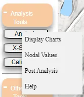
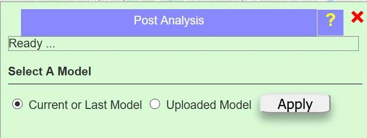
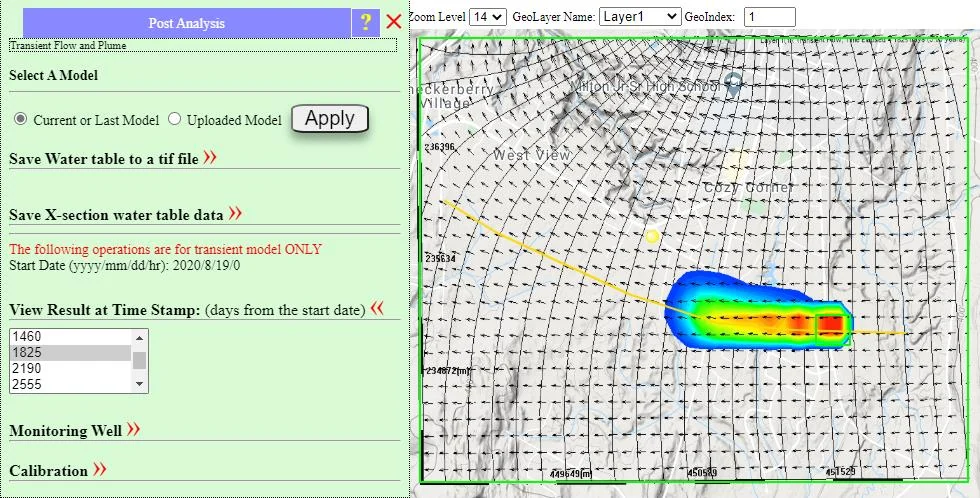
The Post Analysis tool allows us to examine the results of a previously executed simulation (steady or unsteady; just flow or flow and transport, etc.) without having to re-run the model. This is especially useful for simulations that take a long time to run. To access the Post Analysis tool, go to Analysis Tools, then Analysis, then Post Analysis (Figure 84). A warning window prompt will appear; click OK. You now see a window that provides an option as to the model results you wish to use. We will choose Current or Last Model (see Figure 85) to examine the transient model from Section 8.Click APPLY and a warning window regarding clearing the current model comes up and you click OK. The window you see in Figure 86 comes up and you will find that if you click the chevron next to View Result at Time Stamp it will reveal where it is now possible to select from the drop down menu the simulated results for the time step of interest. After clicking APPLY you will be greeted by the warning (if
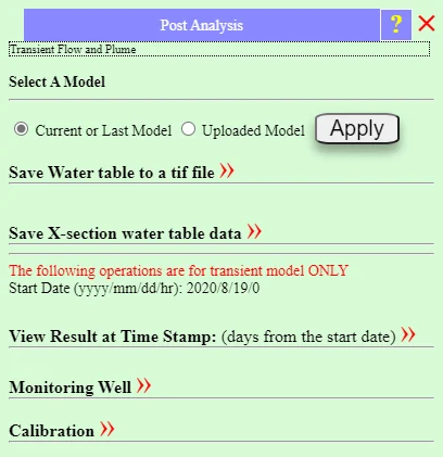
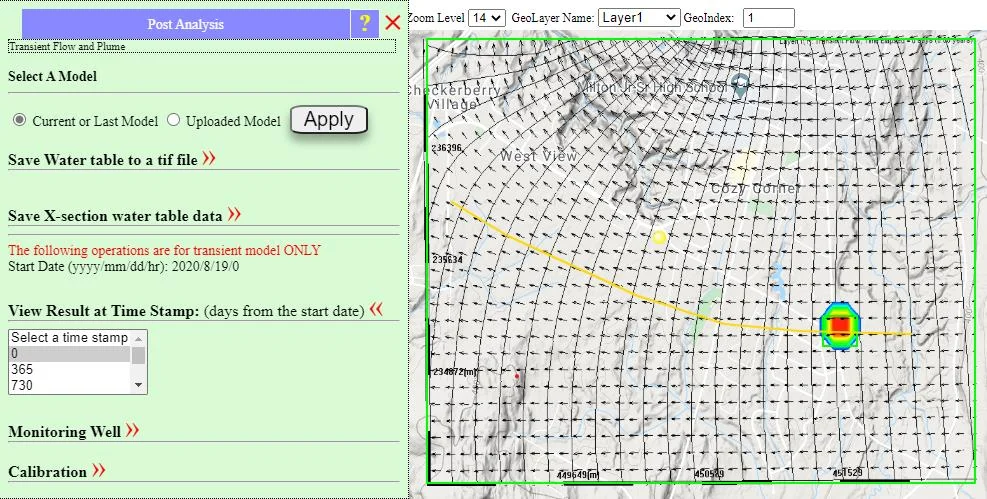
you select other than the last time step). Now Figure 87 will appear. If we select another time-step, again click Apply and wait, we will see updated results in the map display (Figure 88). The Post Analysis tool can also be used to: save the water table for a particular time-step; save the water table along a cross-section for one or more time-steps; compare the transient model results to temporal static water level data (calibration); or extract head and/or concentration time-series results from a monitoring well.
9.2 Map Display Options
IGW-NET has many options for visualizing computed results, especially the plan view results shown in the
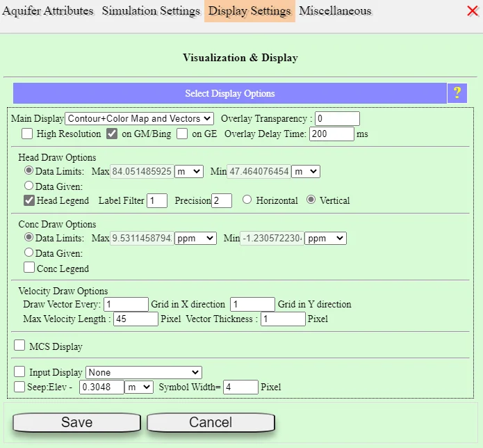
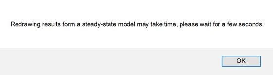
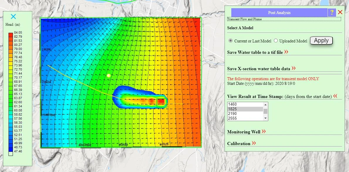
map display. We have seen the contouring option with superposed velocity vectors. In this section we will explore a few other possibilities. To access the control panel for selecting visualization options you go to DomainAtt and then select Display Settings. The control panel will appear as shown in Figure 89. The primary change you might make here is to the Data Limits of the Head Draw Options. The Max will be the highest observable contour and Min will be the smallest. Changes to the Velocity Draw Options could also be of interest. Clicking the box next to Head Legend will add a head legend when you click the SAVE button. Next click on the Contour and Vectors button (the little v to the right of this window). Select the particular option that best fits your needs. When finished click on the SAVE button. The message presented in Figure 90 appears. Click OK to continue. Next we add color to the plot and get Figure 91 . One aspect of this choice is that we lose the geographical map features. But we can return to the Display Settings menu and change the Overlay Transparency (top-right portion of the menu) to a value larger than 0 (up to 100 percent transparency). Or we can temporarily hide the output overlay by clicking Other
Tools, then HideOverlay. To toggle back to having the model output shown, click the ShowOverlay button that now occupies the spave the HideOverlay button once did (and so on and so forth).
§ 10 Growing with IGW-NET
We have now covered many of the steps for setting up a basic model using default settings and values and modeling more details in an “incremental” manner. Many of the steps along the way can be altered or customized using the different options available or by using the Data Center data or user data as inputs. This manual is not meant to be all-encompassing or completely exhaustive of the complete capabilities of IGW-NET; in fact, IGW-NET’s capabilities and functionalities are constantly expanding and improving, so a manual of that nature would become quickly outdate. However, this document should give you an excellent foundation to become more and more experienced as a IGW-NET user. So how can you “grow with IGW-NET” after completing this document, you might ask. There are many resources available.
10.1 Situational Help Pages
As previously mentioned in Section 3.2, for all menus and input options, there are ? buttons that launch situational help pages for the particular input/option/setting you are trying to use. This includes information how “What is it” and “How to use it”, among other items. You will notice that many of the buttons underneath the main list boxes (Conceptual Model Tools, Simulation Tools, etc.) which launch submenus (e.g., Zones, or Lines) have an option called Help. Clicking on these Help options will launch a Real-time Help Page with instructions for how to use the menu / button palette.
10.2 Main Menu Help Pages
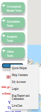
Beneath the Other Tools list box in the IGW-NET modeling environment is a button called Help (see Figure 92). This provides access to the Quick Helper menu (the window found when first loading the platform page, used by first-time users) and My Account, which we discussed in Section 2.
10.2.1 My Account Page
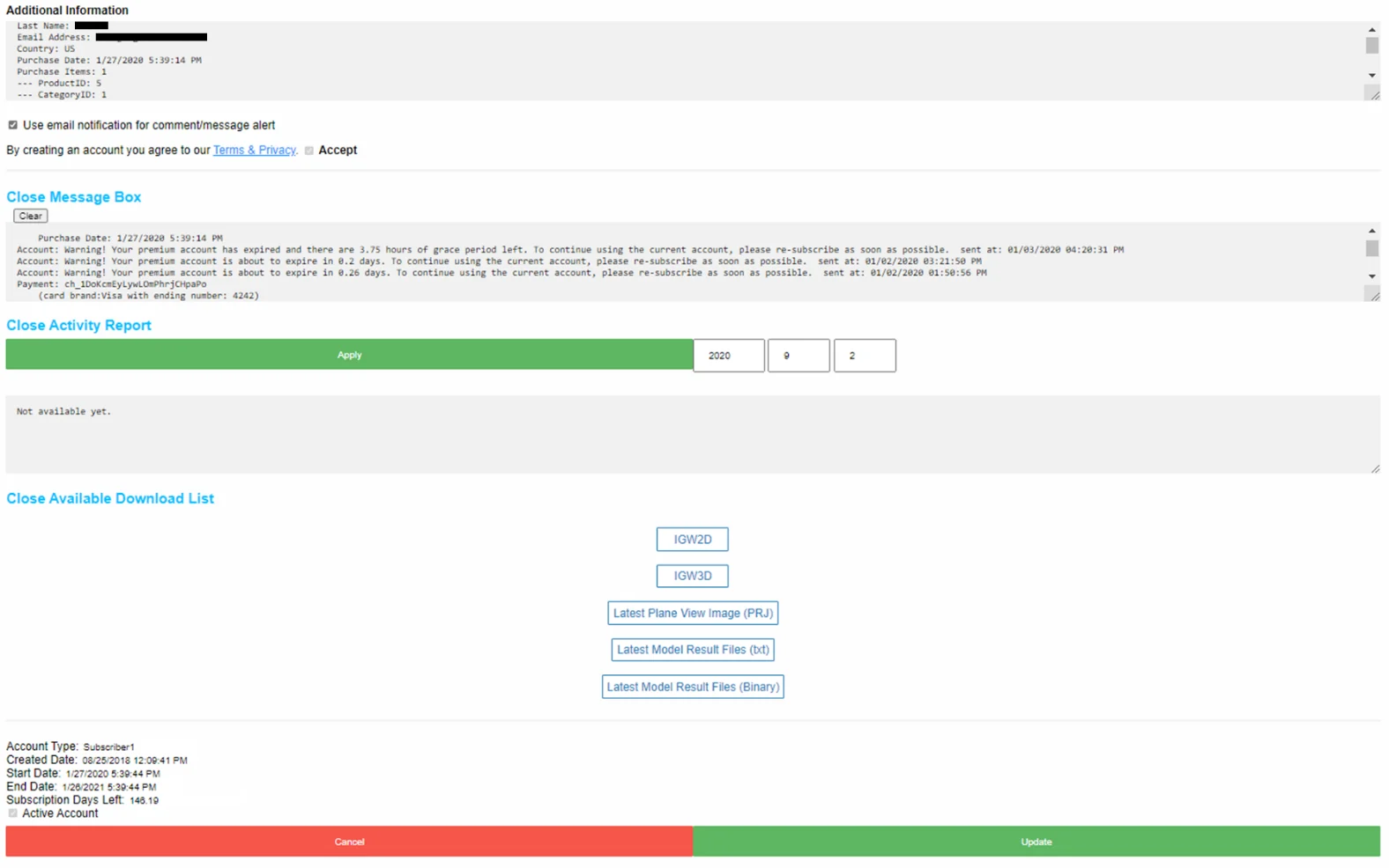
When you successfully log into My Account, you will see the same fields for editing that were included in the Hydrosimulatics Sign Up Form (Section 2), but also additional features related to user accounts. In the bottom-left, information related to the Account Type, the date the account was created, and the starting and end dates for premium subscriptions (unlimited grid/computational settings) . Users may also directly view messages sent to their account emails and view recent activity by using the hovering over and clicking the ‘View Message’ or ‘View Activity Report’ hyperlinks just above the Account Type information (see Figure 93). If the ‘View Activity Report’ option is selected, the user must specify a date (year, month, day) from which to extract an activity report, then click ‘Apply’. The report file will be outputted to the text box just below. If the ‘Click Available Download List’ option is selected, four clickable icons will appear. • Clicking ‘IGW2D’ allows users to download/run the free-to-use IGW2D.exe application file on the local desktop. • Clicking ‘Latest Plane View Image (PRJ)’ downloads/opens a *.bmp image file of the latest model results (plan view display of head contours, velocity vectors, particle pathlines, etc.). • Clicking ‘Latest Model Results Files (txt)’ downloads/opens a IGW-NET model result file which includes the model structure (number of cells, cell size, etc.) and model outputs for each cell (cell index, head, conductivity, bottom and top aquifer elevation). See Figure 1 8 for an example. • Clicking ‘Latest Model Result Files (Binary)’ downloads a *.bin binary file containing model results from the last time-step (or steady-state results), specifically, the 2D or 3D head distribution and solute concentration distributions. This *.bin file can be uploaded to IGW-NET to provide initial/boundary conditions for a new model as described Section 3.6 (feature coming soon).
10.2.2 Bug Reporting / Commenting
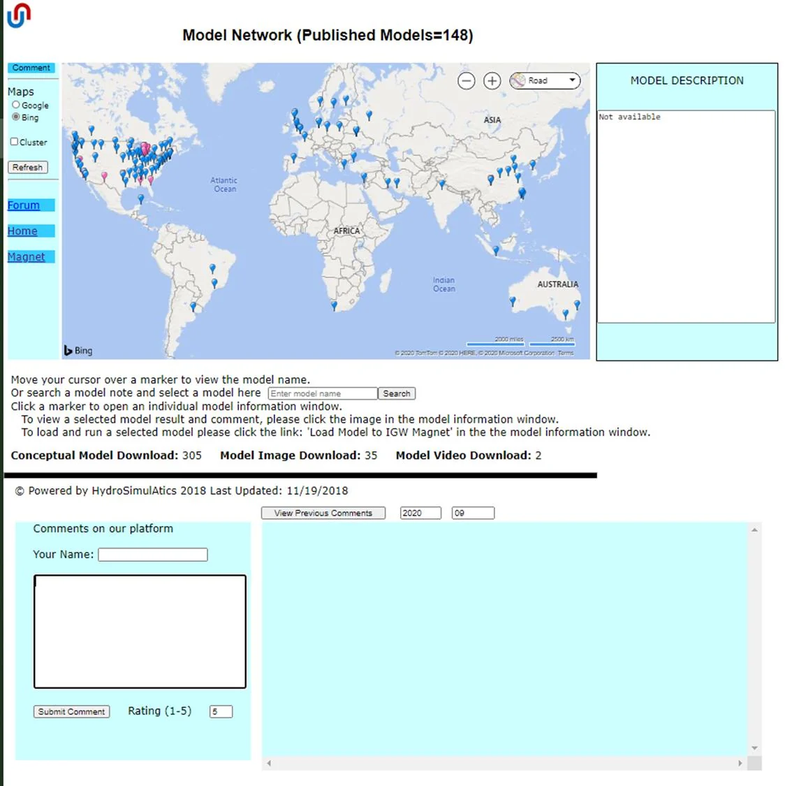
Click the Bug Reports and Comments link shown in Figure 92 to open MAGNET Model Network page in a new browser tab (see Figure 94). The map shows the current set of published MAGNET models as markers or “push-pins”. Clicking on a marker opens a small window where more details about the model area available. At the bottom of the Model Network page is a Comment box where you can post comments or report “bugs” (technical issues). You can view previous comments from a particular year and day using the text fields and View Previous Comments button that is provided.
10.2.3 Live Chat
Also seen in Main Menu Help Page is a link to MAGNET’s Live Chat support page. This page can also be accessed through the magnet4water.net home page by navigating to the Support tab and clicking Live Chat (see Figure 95). The resulting subpage is shown in Figure 96. Click Go To Live Chat to initiate a session.

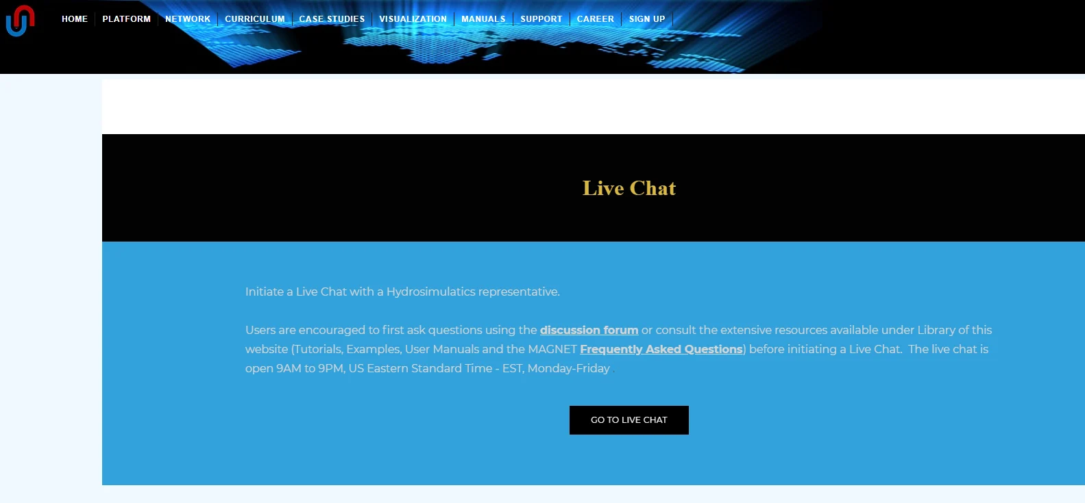
A representative will be alerted via email of your new Live Chat session and will join you as soon as possible.
10.3 Discussion Forum
Also available through the Support tab/header of the magnet4water.net webpage is a Discussion Forum link. Clicking this will result in the webpage shown in Figure 97. Use the Search bar to look for relevant previously posted material, or start a new post.

10.4 Tutorials and Demos
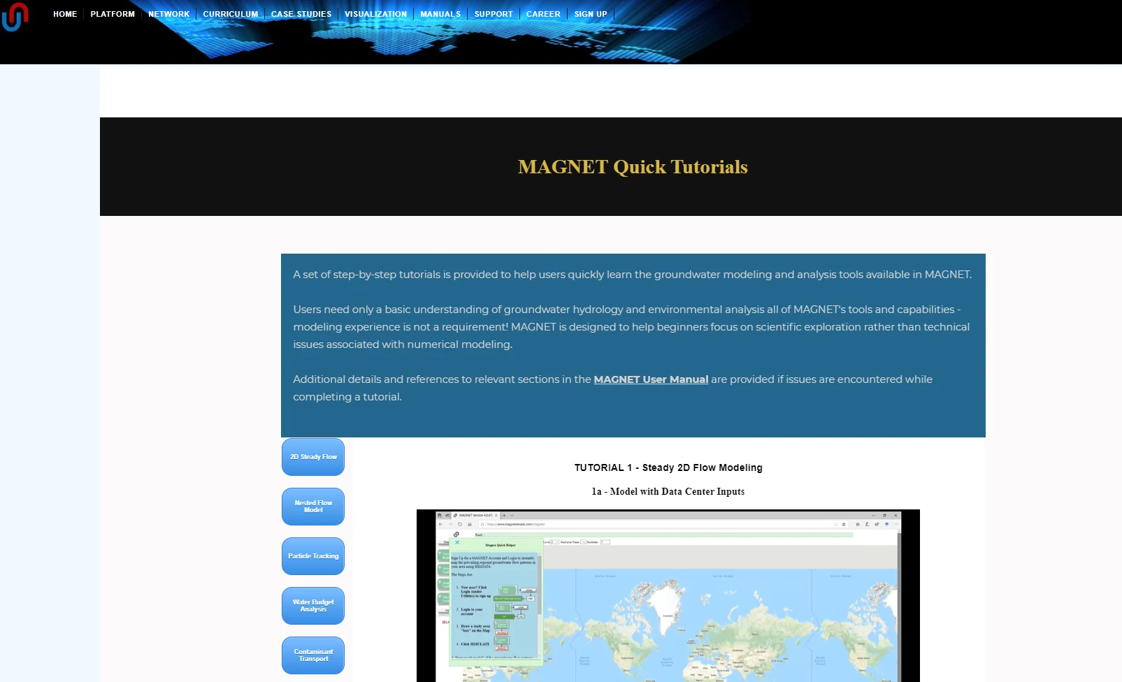
About 20 ‘quick and easy’ tutorials are available that focus on one particular aspect of modeling flow and transport using IGW-NET. Most of these tutorials include a real-time screen capture video; all tutorials include step-by-step written instructions with annotated graphics to follow. You can access the tutorials at the magnet4water website under the Manuals header (see Figure 98).
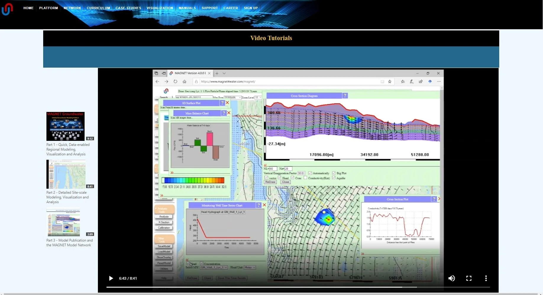
Within the same Manuals header as the Quick Tutorials is a link to video demonstrations of a site in northern Michigan, United States. This includes a regional model and nested local model; flow calibration and transport modeling; and 2D and 3D flow (see Figure 99).
10.5 MAGNET Technical Support
You can email support@magnet4water.net if you encounter any bugs or issues that cannot be troubleshooted using the existing documentation or forums.
§ A Appendix: Structure of Model Windows
Structure of Model Windows