The quick read — 2 minutes
- Use full concentration transport when particle tracking (Ch. 11) is not enough. Particles give you advection; full transport adds dispersion, sorption, decay, and reactions — and gives you dissolved concentration values (ppm, mg/L) at specific locations over time. Reach for this chapter when you need actual concentrations to compare to MCLs, when the contaminant degrades or sorbs meaningfully, when multiple species interact (PCE → TCE → DCE → VC), or when density couples transport back to flow (seawater intrusion).
- Transport auto-activates. The moment you assign a non-zero concentration anywhere in the model — a source zone, a zone override, a well injection, a polluted stream, a recharge value — IGW-NET starts simulating transport. No separate "enable transport" checkbox.
- Contamination can enter from everywhere — but only where water is flowing IN. Internally: source zones (continuous or pulse), zone concentration overrides, initial concentration fields. Externally: injection wells, polluted losing streams and lakes, polluted recharge, and any boundary where inflowing water carries concentration (prescribed head, prescribed flux, head-dependent). Features that only remove water — one-way drains, extraction wells — are categorically never sources.
- Five physical processes govern how a plume evolves: advection (moves with groundwater — the process particle tracking covers), dispersion (spreads from velocity variations), diffusion (Fickian mass transfer, usually minor), sorption (reversible mass-exchange with soil, retards the plume), decay (first-order mass loss to biodegradation or radioactive decay). You control each independently.
- Mind numerical dispersion. Finite-difference transport solvers represent concentration as one average value per cell; on coarse grids this averaging adds plume spreading that looks like dispersion but isn't. It over-predicts plume extent (conservative) and under-predicts peak concentration (not conservative). Fine for screening; for quantitative regulatory or litigation work, refine the grid or use nested submodels, and pair the plume with particle tracking as a diagnostic.
- 2D is fine for screening; 3D becomes important for calibration. A plan-view 2D transport simulation — without vertical dispersion or diffusion — is a reasonable first look at a site and is often slightly conservative on horizontal plume extent. But field measurements are inherently 3D (each well screen samples a specific depth, and concentrations typically vary substantially with depth), so comparing a 2D simulation to measured data usually produces mismatches that no parameter adjustment can resolve. When your work moves from exploration to calibration or prediction, switch to sublayered 3D — enable the Water Table as Top flag and add 5–10+ sublayers. IGW-NET's efficient workflow: run 2D first to get the water table, then turn on sublayers; the platform automatically uses the most recent water-table result as the top of the uppermost sublayer, avoiding expensive free-surface iteration.
- Multi-species reactions via MT3DMS handle everything from simple first-order chain reactions to full biogeochemistry. Five predefined modules: BTEX instant aerobic, BTEX kinetic with multiple electron acceptors, PCE sequential dechlorination, combined PCE/TCE aerobic-plus-anaerobic, single-pair instant electron-donor/acceptor.
- Dual-domain transport for fractured rock, macropores, karst, or strongly heterogeneous aquifers — splits the medium into a mobile (flowing) domain and an immobile (stagnant) domain exchanging by diffusion. Reproduces the long slow-tailing breakthrough curves that single-domain cannot.
- SEAWAT for variable-density problems — seawater intrusion, brine migration, thermal plumes. Concentration couples back into flow through density effects.
- Read transport results via plume plan views (colored contours), cross-sections (vertical structure), breakthrough curves at monitoring wells (concentration over time), and the transport water balance (mass in, mass out, mass in storage).
12.1 Transport Auto-Activates
Unlike most groundwater modeling platforms, IGW-NET has no separate on/off checkbox for contaminant transport. The moment you assign a non-zero concentration anywhere — a source zone polygon, a zone override, a well's injection concentration, a polluted stream's concentration, the recharge concentration field — transport simulation activates automatically and the solver begins tracking the resulting plume.
12.1.1 Why auto-detection matters
This design choice reflects a practical observation about how modelers actually work. If transport is a checkbox, users routinely forget to turn it on after defining a source, and then wonder why the plume isn't appearing. Conversely, leaving transport "on" with no sources wastes computation on a trivial no-transport solution. Auto-detection eliminates both failure modes: no source means no transport simulation; any source means transport is simulating. The user experience matches the physics — transport happens if and only if there's something to transport.
12.1.2 How to tell if transport is active
Three indicators confirm transport is running:
- The Simulate button's behavior — if transport is active, the simulation takes modestly longer than flow-only and the resulting animation includes plume migration.
- The Analysis Tools — concentration charts, breakthrough curves, and the transport mass balance become available only when transport is active.
- The automatically-generated model description (via the Intelligent Reporting System) — explicitly states "Contaminant transport is active" or "No contaminant transport," with the list of detected sources.
If you defined what you thought was a contamination source and you don't see a plume, the usual cause is that the source has concentration of zero (forgetting to fill in the value), or the source is specified in the wrong place (e.g., a zone polygon where you meant a source zone, or a well with Q > 0 but the concentration field left blank). The Intelligent Reporting System's description of your model will flag which sources the platform sees; compare that list to what you intended.
12.2 Where Contamination Comes From
The single most important concept in this chapter: contamination can enter your model from many distinct pathways, and getting the right pathway right is often more consequential than getting the physical processes right. This section presents the catalog in two voices — the applied-practitioner voice (how an EPA manager, consultant, or site investigator thinks about contamination) and the modeler voice (how it maps to IGW-NET's boundary-condition controls).
12.2.1 The applied view — contamination as it actually happens
Real-world contamination enters aquifers through recognizable pathways. A site investigator or EPA manager doesn't think in terms of boundary conditions; they think in terms of what actually happened at a site.
| Applied category | Examples | Release pattern |
|---|---|---|
| Spills and leaks at or below ground surface | Leaking USTs, pipeline ruptures, accidental releases, dry cleaner solvent spills | Typically continuous while the leak is active; becomes historical (pulse-like) once sealed |
| Long-term source areas | Landfills, industrial dump sites, stockpiles, unlined lagoons, long-term surface impoundments | Continuous, often for decades |
| Agricultural and land-use sources | Fertilizer leaching, pesticide percolation, concentrated animal feeding operations, septic fields | Continuous to seasonal; often spatially distributed rather than a single point |
| Polluted surface-water bodies recharging the aquifer | Losing streams downstream of a contaminated reach, leaking lagoons, artificial recharge basins with poor-quality water | Continuous when the feature is losing; can reverse if conditions change |
| Contaminated rainfall and atmospheric deposition | Nitrogen deposition near agricultural areas, acid rain, near-facility atmospheric fallout | Continuous spatially uniform or distributed; follows climate patterns |
| Injection wells | Remediation injection wells (adding treatment reagents), disposal wells, tracer tests, aquifer storage and recovery with poor-quality water | As defined by the operations schedule — typically transient |
| Regional upgradient plumes entering the domain | Contamination originating outside your model, migrating in from the regional boundary | Continuous inflow as long as the upgradient source is active |
| Historical pre-existing contamination | Old spills you didn't know about, legacy plumes already present at the start of your simulation period | Pulse loading at t = 0 — an initial condition, not an ongoing source |
12.2.2 The modeler view — the same pathways as boundary conditions
Inside the simulator, every source in the applied list above is expressed as one of five modeler-recognizable configurations. The vocabulary is the same you'll see in IGW-NET's dialogs, in published MODFLOW/MT3DMS documentation, and in any groundwater-modeling textbook.
| Modeler configuration | What it is, in transport terms | Applied examples it covers |
|---|---|---|
| Internal source term (inside the aquifer) | A continuous or pulse release defined within a polygon on the domain — the solver adds mass at that location at the specified rate. Also called "source zone" in the interface. | Leaky tanks, spills, landfills, dump sites, areal agricultural sources, any contamination released inside the modeled aquifer |
| Initial concentration field (at t = 0) | Concentration assigned to specific zones or cells at the start of the simulation — a "pre-existing plume" specified before any transport advancement. | Historical contamination present at the start of the modeling period; pulse loading from a past spill already complete |
| Well injection with non-zero concentration | A well's Q > 0 combined with a specified concentration. Each time step, the solver adds the volumetric inflow × concentration to that cell. | Injection wells for remediation or disposal, tracer tests, ASR with poor-quality water |
| Recharge with non-zero concentration | The recharge attribute field has a concentration assigned. Recharge always flows into the aquifer from above, so the recharge concentration is always added at the top surface. | Polluted rainfall, atmospheric deposition, agricultural runoff, leaking septic at the surface |
| Head-dependent flux boundary with inflowing water carrying concentration | A two-way stream, two-way lake, or general head-dependent boundary carries concentration when the computed flow direction at that segment is into the aquifer. When the feature is losing, the external concentration enters; when gaining, nothing is added. | Polluted losing streams, polluted leaking lakes, contaminated reservoirs, surface-water sources that intermittently recharge the aquifer |
| Prescribed-head boundary with inflowing water carrying concentration | A boundary (types 1, 2, 3) where the solver computes inflow from the prescribed head; inflowing water carries the boundary's assigned concentration. Like the head-dependent case, this operates only at segments where flow is computed to go into the domain. | Regional upgradient plumes entering through a prescribed-head boundary representing a larger aquifer; contaminated lake modeled as prescribed head |
| Prescribed-flux boundary with concentration | A boundary (type 7) where flux into the domain is prescribed directly. Concentration is assigned to that inflow. | Known inflow with measured or estimated concentration, e.g., from a regional groundwater model supplying boundary conditions with known water quality |
12.2.3 The rule, in both voices
The single rule that ties everything together — expressed twice, once for each audience — determines whether any given feature can be a source.
Applied voice. Contamination can enter the aquifer only where water is flowing IN. A losing stream carrying dirty water — yes, that's a source. A gaining stream that's the aquifer's outflow — no, that's a sink, even if the stream is polluted. An injection well adding contaminated water — yes. An extraction well removing contaminated water — no, that's carrying contamination away, not introducing it. Polluted rainfall infiltrating into the aquifer — yes. A one-way drain removing water — no, categorically. The test is: is the feature putting water INTO the aquifer? If yes, whatever concentration that water carries becomes a source. If no, the feature cannot introduce contamination.
Modeler voice. A boundary segment or feature contributes mass to the transport equation as a source only when the computed (or prescribed) flow direction is into the domain at that segment. A head-dependent boundary is a source during inflow time steps and a sink during outflow time steps — the role is instantaneous and can switch from one time step to the next. A one-way drain has "flux out only" enforced structurally, so it cannot ever be a transport source. Extraction wells, similarly, have Q < 0 — their mass contribution to the transport equation is negative, subtracting existing aquifer mass at the well rather than adding new mass.
12.2.4 Features that are categorically never sources
This list exists to prevent a common mistake. The following features cannot be contamination sources, regardless of how they are configured:
| Feature | Why it cannot be a source |
|---|---|
| One-way drain (polyline type 6) | Flow direction is structurally one-way out of the aquifer. Water cannot flow from the drain into the aquifer even in principle. |
| One-way drain polygon (lake/wetland configured as one-way) | Same as above — polygon variant of the drain. |
| Extraction well (Q < 0) | Removes water from the aquifer. If that water is contaminated, the contamination is removed; no new contamination is introduced. |
| "Calculate Flux" polyline (type 4) | A measurement line only — imposes no boundary condition of any kind. |
| "None" polyline (type 0) | Display annotation only — no hydraulic or transport role. |
If you find yourself trying to introduce contamination through one of these features, you need a different feature. A polluted drainage ditch that represents contaminated water recharging the aquifer should be modeled as a two-way stream or as a head-dependent polygon, not as a one-way drain. An extraction well that's part of a recirculation system where treated water goes back in should be two wells (extraction + injection), not one reversible well.
12.3 Setting Up Sources
This section walks through the mechanics of defining each source type. The applied and modeler categories from §12.2 map to specific dialogs and controls in IGW-NET.
A plan-view 2D transport simulation is a legitimate starting point for exploring a site — it's fast to set up, reasonable for screening, and slightly conservative on horizontal plume extent (because no vertical dispersion carries mass away from the plume axis). You can learn a lot from a 2D model without going further. But if you plan to calibrate against real field data or to defend predictions against observed concentrations, 3D becomes important. Real monitoring wells sample specific depths, not aquifer-averages, and concentration usually varies substantially with depth — so a 2D simulation compared to 3D measurements produces systematic mismatches that no parameter adjustment can resolve. See §12.4.7 for how to switch to sublayered 3D when you reach that stage.
12.3.1 Areal source zones — continuous and instantaneous
The most common source configuration in practice: an area of the domain where contamination is released, either continuously or as a pulse at t = 0.
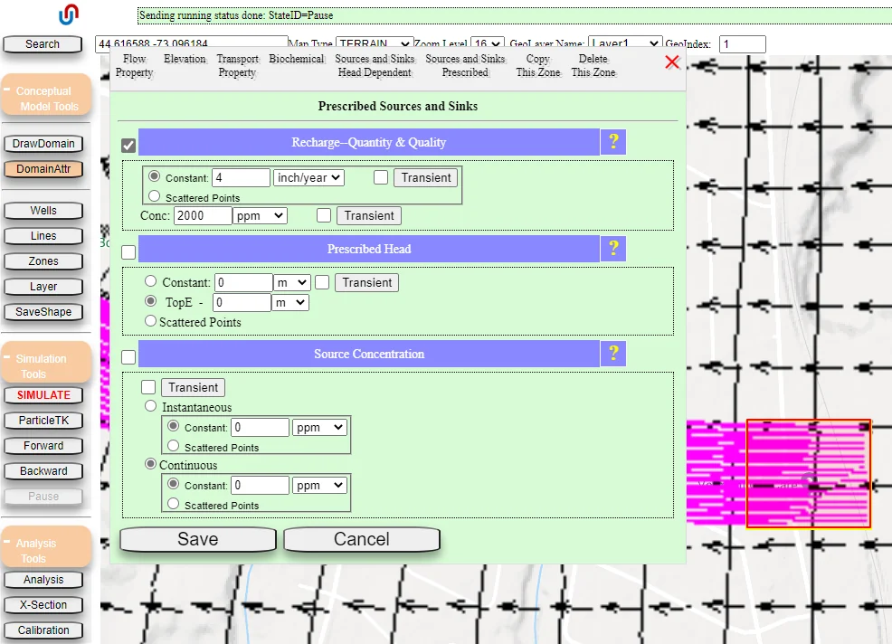
Draw a source zone polygon
Use Draw Zone to create a polygon covering the source area (a landfill footprint, a leaking tank's estimated affected area, a spill footprint). Precise geometry matters — the cells under the polygon are where mass is added.
Open Zone Attributes → Sources and Sinks → Prescribed
In the Zone Attributes dialog, navigate to the Sources and Sinks tab, Prescribed subtab. This is where concentration sources are defined.
Assign a concentration
Enter a non-zero concentration (ppm or mg/L, per your unit setting). This activates transport automatically.
Choose continuous or instantaneous
Select the release pattern. Continuous releases mass at the specified concentration throughout the simulation — appropriate for ongoing spills, active landfills, leaky tanks still in service. Instantaneous (pulse) releases the entire mass at t = 0 and then stops — appropriate for a one-time historical spill or a tracer test.
12.3.2 Zone concentration overrides — initial conditions within a zone
Distinct from the source-zone release pattern above, a zone can also have a concentration override that sets the aquifer's initial concentration within that zone. This is how you represent a pre-existing plume at t = 0 — a legacy plume you're starting to model with some characterization already known.
In the Zone Attributes dialog, the concentration field assigns an initial value at every cell inside the zone. If you specify a source polygon for ongoing release plus a zone override for initial concentration, you get both effects: contamination already present at t = 0, plus continued release from the source.
12.3.3 Wells with injection concentration
An injection well with a non-zero concentration adds mass at the well cell each time step. Chapter 6 §6.4 introduced the well record with its 13 fields; for transport sources, the relevant field is Conc_ppm:
- Set
Q > 0(positive, meaning injection). - Set
Conc_ppmto the concentration of the injected water. - The solver adds mass at a rate of
Q × Conc_ppmat the well cell, each time step.
For an injection well with a time-varying pumping schedule (Ch. 9 §9.4), the injection concentration can likewise be time-varying — e.g., modeling an in-situ remediation system where reagent concentration changes with operating procedures.
12.3.4 Polluted rain recharge
Recharge always enters the aquifer from above, so a non-zero concentration assigned to the recharge field represents contamination dissolved in infiltrating precipitation. This handles:
- Agricultural fertilizer and pesticide leaching — often spatially distributed by land use (assign via zone overrides to give different recharge concentrations to different land-use categories)
- Atmospheric deposition from nearby sources — typically spatially uniform unless concentrated dispersion patterns are modeled
- Acidic or chemically-altered recharge from surface disturbance
- Leaking septic systems operating as areally distributed surface-layer sources
Where recharge concentration varies spatially (land-use patterns, distance from a surface source), use zones or uploaded rasters to carry the spatial pattern.
12.3.5 Polluted streams and lakes (two-way features)
For a polluted stream or lake to contribute as a source, three conditions must hold: (1) the feature is configured as two-way head-dependent (not one-way drain); (2) the feature has a non-zero concentration in its attributes; (3) the computed flow direction is into the aquifer (the feature is losing water at that segment).
In the Edit Polyline Attributes dialog for a two-way stream (type 5), or the Zone Attributes dialog for a two-way head-dependent lake polygon, you will find a concentration field. Fill it with the stream or lake water's contamination level. The platform handles the rest — during time steps when the feature is losing, contamination enters the aquifer; during time steps when the feature is gaining, no mass is added (the aquifer's own concentration is carried out instead).
12.3.6 Prescribed-head, prescribed-flux, and transient-head boundaries
Any boundary segment where water enters the aquifer can carry concentration. For prescribed-head polylines (types 1, 2, 3) and the head-from-transient-file polyline (type 8), the dialog includes a concentration field that applies to any inflowing water. For prescribed-flux polylines (type 7), the concentration applies to the specified inflow flux.
The platform handles the direction test automatically — it will apply the concentration only at segments and time steps where water is flowing in, and never at segments or times where water is flowing out.
If contamination is entering your model from beyond the domain boundary — a regional plume migrating in from a known source area outside your model — a prescribed-head or head-dependent boundary with assigned concentration is the standard representation. Set the concentration to the contamination level at the upgradient edge of your domain (from field data or from a larger regional model). The platform handles the rest: the boundary acts as a source for as long as heads drive water into your domain through that segment.
12.4 The Five Physical Processes — and How to Invoke Them in IGW-NET
Once you've defined your sources, five physical processes govern how the resulting plume evolves. Each has a distinct physical mechanism; each is controlled by specific fields in IGW-NET with specific defaults. This section walks through each process as the platform handles it: what you do to turn it on, what you see when you do, and the IGW-NET-specific judgment calls that decide whether your parameter value is right for your problem.
Two organizing facts that recur for every process:
- Transport is auto-activated by concentration sources (§12.1), but each individual process must be enabled separately. The platform's default transport simulation is advection-only. Dispersion, diffusion, sorption, and decay are opt-in — you activate each by checking its flag in the Aquifer Attributes dialog and supplying parameters.
- When a process is off in IGW-NET, its parameters don't matter. The platform ignores αL if the dispersion flag is off, ignores Kd if the sorption flag is off, and so on. Setting non-zero values without checking the activation flag is a common "why isn't this working?" source of confusion.
12.4.1 Advection — always on
Advection is the only one of the five processes that is always active in IGW-NET. The platform transports dissolved mass with the local groundwater velocity without any flag to enable it and without any parameter to tune — it is the baseline that the other four modify. This matches the physics: you cannot have dissolved transport without the bulk flow of water carrying it.
Because advection velocity comes directly from the flow solution, your transport results are only as good as your flow solution. If your hydraulic conductivity is wrong, plume arrival times will be wrong proportionally. If your regional gradient is off, your plume goes in the wrong direction. For this reason, the standard IGW-NET transport workflow is: calibrate flow first (Ch. 17), verify heads match observations, then add transport. Trying to fit transport data with a poorly calibrated flow field burns parameters on compensating for flow errors.
12.4.2 Mechanical dispersion — the Dispersivity dialog
Dispersion represents plume spreading from velocity variations smaller than the grid resolves: pore-scale variability, intra-cell heterogeneity, velocity differences between streamlines. In IGW-NET, you invoke it through the Dispersivity controls inside the Aquifer Attributes dialog. The field carries four values internally — an activation flag and three dispersivity coefficients.
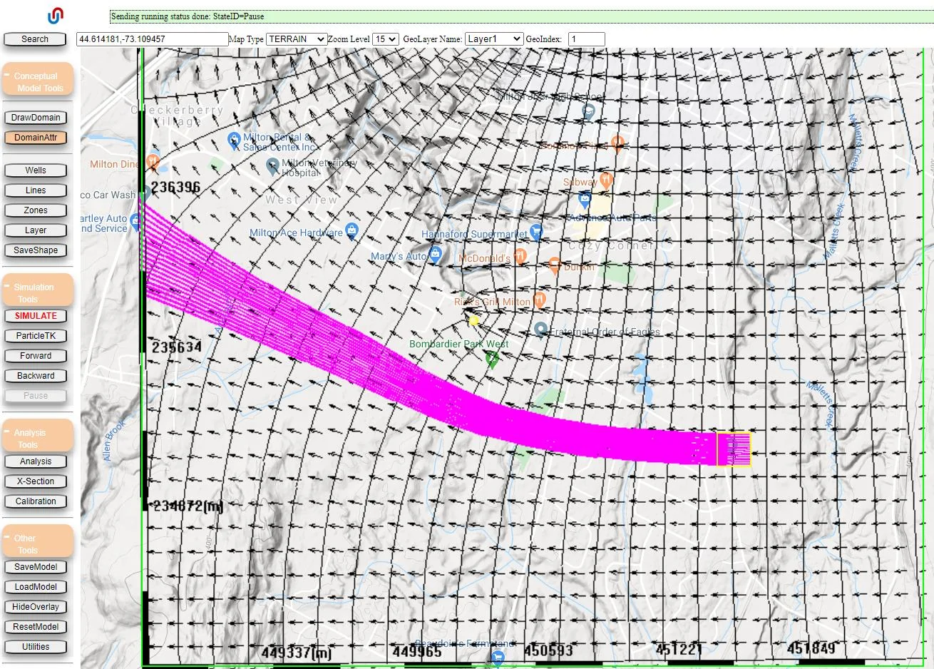
| Field | What you enter | IGW-NET default |
|---|---|---|
| Dispersion active (flag) | Off or on | Off — new models have no dispersion by default |
| αL (longitudinal, along flow) | Meters — the principal parameter, usually the largest of the three | 0 m |
| αT (transverse horizontal, perpendicular to flow) | Meters — commonly set to αL/10 | 0 m |
| αV (transverse vertical) | Meters — commonly set to αL/100 to αL/1000 in layered systems | 0 m |
The platform's default of zero-and-off is deliberate: a new user's first model gives them a pure-advection plume that is easy to interpret visually, and they add dispersion only when they decide their problem calls for it. The visual consequence of turning dispersion on: the plume becomes blurrier at its edges, concentrations at the leading edge drop below the source value, and the plume envelope grows with the square root of travel distance rather than staying as a sharp advection front.
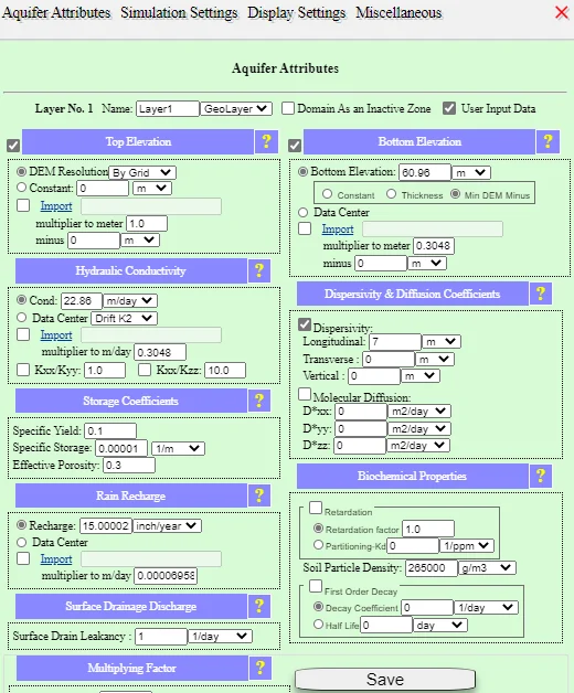
Choosing a value for αL: the practical approach in IGW-NET is to pick a value appropriate for your plume's spatial scale, simulate, and compare the simulated plume's spread to whatever observational data you have. A rule of thumb: αL is typically a few percent of plume length. If your plume is 500 m long, αL in the 5-50 m range is reasonable; if the simulated plume looks too sharp compared to observations, increase αL; if too diffuse, decrease.
| Plume scale | Starting αL | Rule of thumb |
|---|---|---|
| Column/bench test | 0.01 – 0.1 m | ~1% of flow path length |
| Tracer test (tens of m) | 1 – 10 m | ~10% of tracer travel distance |
| Site-scale plume (hundreds of m) | 10 – 50 m | ~5-10% of plume length |
| Regional plume (kilometers) | 50 – 200 m | ~5% of plume length |
Setting αL to zero in IGW-NET does not eliminate plume spreading — numerical dispersion from the grid-based advection scheme will still produce spreading, sometimes substantially more than the physical dispersion you just turned off. On a coarse grid this numerical dispersion can dominate. The next subsection covers why this happens, how to diagnose it, and what to do about it.
12.4.3 Numerical dispersion — when the grid spreads the plume
After you set up physical dispersion with αL, αT, αV, your simulated plume will always spread somewhat more than those values alone predict. The additional spreading is numerical dispersion, and it arises from the fundamental way finite-difference transport solvers represent concentration: as a single average value per cell.
Why it happens — the averaging effect
Concentration inside a real plume varies continuously in space. A finite-difference solver must collapse that continuous distribution into one number per cell — the cell-averaged concentration. When a cell is large relative to the plume's features, averaging over the cell smooths out concentration gradients that really exist on smaller scales. Every time the solver advances contamination across a cell boundary, it re-averages the receiving cell's contents; each averaging step blurs the plume a little more. The cumulative effect over many cells and many time steps is plume spreading that looks like dispersion but comes from the grid, not the physics.
Two consequences are worth understanding because they point in opposite directions:
- Plume extent is slightly over-predicted. Numerical dispersion pushes the plume's leading edge a bit further than physical dispersion alone would, because mass has been smeared ahead of the true front. In a regulatory context, this is conservative — the simulated plume reaches receptors earlier and spreads wider than reality. If your question is "does the plume reach this receptor?", a coarse-grid simulation is likely to say yes more often than reality.
- Peak concentration is under-predicted. The same averaging that smears the leading edge also dilutes the plume core — the same total mass is distributed across a wider and flatter plume, so the peak value is lower than it should be. If your question is "does concentration exceed the MCL at this well?", a coarse-grid simulation may report no even when the true concentration exceeds the threshold.
A single transport simulation on a coarse grid tends to give you a conservative answer for plume extent and a non-conservative answer for peak concentration. This asymmetry matters for how you use the model. "How far does the plume reach?" — coarse is often fine, usually errs on the safe side. "What peak concentration will the well see?" — coarse is often wrong in the dangerous direction, under-predicting peaks. Know which question you're answering, because the grid-resolution needs are different.
When is numerical dispersion acceptable?
For screening-level analysis — preliminary site assessment, go / no-go evaluation, is-there-a-problem questions — numerical dispersion's effects are usually acceptable because you're looking for order-of-magnitude understanding, not precise concentrations. The conservative bias on plume extent is often helpful at this stage. Run a coarse simulation, get a fast answer, identify where to invest more effort.
For quantitative work — regulatory compliance demonstration, remediation design, legal defense — numerical dispersion must be controlled. The remedies in IGW-NET:
Remedies in IGW-NET — in order of effort
| Remedy | What it does | When to use it |
|---|---|---|
| Refine the grid globally | Increase the grid resolution in Simulation Settings (e.g., NX from 40 to 80 or 160). Smaller cells mean less averaging per cell and less numerical dispersion. Cost: simulation time scales roughly with NX × NY × (sublayers). | First thing to try when numerical dispersion is clearly affecting results. Moderate refinement often resolves most of the problem. |
| Refine locally with a nested submodel | Build a fine-grid submodel (Ch. 13) over the plume area, inheriting boundary conditions from the regional model. Fine grid where it matters; coarse grid elsewhere. | Best approach for site-scale transport within a larger regional context. You get the fine-grid accuracy near the source and receptors without paying for fine grid over the whole domain. |
| Switch transport scheme | IGW-NET offers alternative advection schemes in the MT3DMS transport settings (upstream finite-difference, TVD, method of characteristics, MOC/MMOC/HMOC). More advanced schemes produce less numerical dispersion for the same grid, at higher computational cost. | When grid refinement alone is insufficient or too costly. TVD and method-of-characteristics schemes are particularly effective for sharp plume fronts. |
| Run particles alongside the plume | Particle tracking (Ch. 11) has no numerical dispersion — each particle moves along a computed streamline independently of cell averaging. Running particles and plume from the same source area lets you compare: the particle envelope is the advection-only truth; any additional spreading in the plume simulation is some combination of physical dispersion (what you wanted) and numerical dispersion (what you didn't). | Always useful as a diagnostic — a quick sanity check on whether your plume's spread matches advection plus the dispersion you configured, or whether numerical artifacts are dominating. |
The diagnostic workflow — plume against particles
Because particle tracking has no numerical dispersion, pairing the two analyses is one of the most useful diagnostic techniques in IGW-NET:
Place a particle source matching the contamination source
For a source zone polygon, draw a particle rectangle or polygon over the same footprint. Use ~50-100 particles to get a reasonable envelope.
Run flow + particles + plume simultaneously
Click Simulate. IGW-NET advances flow, particles, and plume together; you see all three evolve on the same map.
Compare the envelopes
The particle cloud marks the advection-only plume envelope — where groundwater would carry mass in the absence of any spreading mechanism. The simulated concentration contours should surround the particle cloud: slightly wider than the particles due to dispersion (if you set αL > 0) and numerical dispersion.
Diagnose grid issues from the comparison
If the plume's outer contour is much wider than the particle cloud and you didn't configure much physical dispersion, numerical dispersion is dominating — refine the grid or switch schemes. If the plume's outer contour closely matches the particle cloud but with a slight widening, numerical dispersion is under control and physical dispersion is doing its intended job.
Each particle in IGW-NET moves along a computed streamline in the velocity field, using its own position rather than a cell-averaged concentration. There's no averaging step, no smearing between cells — the particle is where it is, period. So the envelope of a particle cloud reflects pure advection plus whatever physical dispersion/diffusion you've added via the random-walk option (Ch. 11 §11.8). If you run particles without the random-walk option turned on, you see advection alone — the sharpest possible plume envelope that physics allows, against which any widening in the concentration simulation can be attributed to physical plus numerical dispersion. Chapter 11 covers particles in depth.
12.4.4 Molecular diffusion — rarely the main process
Diffusion is parameterized in IGW-NET by an activation flag plus three directional diffusion coefficients (Dxx, Dyy, Dzz) in the same Aquifer Attributes dialog as dispersivity. Defaults are all zero and off — diffusion is not active in a new model.
For most IGW-NET transport problems, diffusion is the smallest of the five processes and you can leave it at zero without meaningful error. At typical groundwater velocities, dispersion dominates diffusion by two to four orders of magnitude. There are three situations where you should turn diffusion on:
- Very slow-flow systems where you're modeling transport through confining units or aquitards. When groundwater velocity is near zero, diffusion is the main mass-transport process.
- Dual-domain transport (§12.7) — mass exchange between the mobile and immobile domains is driven by diffusion. If you're using dual-domain in IGW-NET, diffusion needs to be active.
- Long-timescale legacy problems — century-scale simulations where even small diffusion contributions can matter.
Typical values when you do need them: 10-5 to 10-4 m²/day in saturated porous media, with temperature correction possible through SEAWAT's viscosity package (§12.8). The default isotropic assumption (Dxx = Dyy = Dzz) is adequate for most purposes.
12.4.5 Sorption and retardation — two parameterization paths
Sorption represents reversible mass-exchange between the dissolved phase and the aquifer solids, slowing plume migration relative to groundwater flow. In IGW-NET, you activate sorption through the Sorption/Decay section of the Aquifer Attributes dialog. The platform offers two ways to specify the same physics — pick whichever matches your available data:
| Parameterization | Fields you fill | Use when... |
|---|---|---|
| Linear Kd (distribution coefficient) | Kd (1/ppm or mL/g) plus soil bulk density (g/m³, default 265,000 — a typical value for saturated granular aquifer material) | You have Kd values from literature tables, partition-coefficient databases, or lab batch tests. The platform computes the effective retardation from Kd and bulk density. |
| Direct retardation factor (R) | R (dimensionless, > 1) | You have R directly from tracer tests, or you want to use a rule-of-thumb R without computing it from Kd. Simpler when only the net effect matters. |
The visual consequence of turning sorption on: the plume moves slower than groundwater velocity would predict. A retardation factor of 5, for example, means the plume's center of mass advances at one-fifth the groundwater velocity. For a pulse release, the plume moves slower and also tails longer (sorbed mass slowly desorbs, maintaining low concentrations after the main body passes). Watch the animated simulation with and without sorption — the difference is immediately visible.
Two IGW-NET-specific choices worth being deliberate about:
- Soil bulk density default (265,000 g/m³). This is the platform's canonical value for saturated granular aquifer material. For rock aquifers or unusually dense/loose material, adjust: sandstone around 250,000, limestone around 270,000, loose alluvium around 180,000. An error here of 20% produces a corresponding 20% error in computed R from Kd.
- Species-specific sorption in multi-species simulations. Each species in a multi-species simulation (§12.5) has its own Kd — PCE sorbs strongly, VC weakly, benzene moderately. A single global Kd for all species is wrong; the Multiple Species dialog has per-species parameters for this reason.
12.4.6 First-order decay — half-life or λ
Decay represents irreversible mass loss — biodegradation, radioactive decay, hydrolysis, or any process that destroys mass rather than just moving it around. In IGW-NET, decay is activated in the same Sorption/Decay section as sorption, with two alternative parameterizations available (just like sorption):
| Parameterization | What you enter | Use when... |
|---|---|---|
| Half-life | Half-life in days (or years — the dialog accepts either with a unit toggle) | You know the contaminant's half-life from literature — most organic compounds and radionuclides are tabulated this way |
| Decay constant λ | λ in 1/day | You have λ directly from fit data, or your reference uses λ rather than half-life |
The two parameterizations are mathematically equivalent: half-life = 0.693 / λ. IGW-NET computes the other when you supply either. Typical half-lives to use:
| Contaminant | Typical half-life | Notes |
|---|---|---|
| Benzene (aerobic) | 10 – 730 days (2 weeks to 2 years) | Fast with oxygen; much slower anaerobically |
| TCE | 3 – 15 years (anaerobic) | Needs anaerobic conditions for meaningful decay in natural attenuation |
| Vinyl chloride | 1 – 5 years | Faster than parent compounds |
| Nitrate (denitrification) | 10 – 1000 days | Highly dependent on electron donor availability |
| Tritium | 12.3 years | Radioactive — fixed regardless of conditions |
| PFAS compounds | Effectively no decay | Use zero or don't activate decay |
First-order decay in the Aquifer Attributes dialog applies the same rate to all dissolved mass, everywhere, all the time. This is an adequate approximation for radioactive decay (always true) and for biodegradation under uniform, non-limiting conditions. It fails for real biogeochemistry — where rates depend on electron acceptor availability, biomass growth, substrate limitation, or pH. When your problem is genuinely biogeochemical, the predefined reaction modules in §12.6 handle the dependencies properly. The choice: first-order decay for simple screening; reaction modules when the chemistry actually drives the results.
12.4.7 2D vs 3D — the sublayer question
Before going further with transport setup, one architectural decision deserves attention: do you need vertical resolution in the plume, or is a plan-view 2D simulation sufficient for your purpose? Both are legitimate; the right choice depends on what you're using the model for.
When 2D transport is appropriate
A plan-view 2D transport simulation — one conceptual layer, one sublayer, no vertical dispersion or diffusion — is a reasonable starting point and often the right final choice. It is:
- Fast and cheap — simulations run in seconds, so you can iterate through source configurations, dispersivity values, and scenarios quickly.
- Slightly conservative on horizontal extent — with no vertical dispersion to carry mass away from the plume axis, 2D plumes tend to be somewhat longer and more concentrated than equivalent 3D plumes. For screening purposes this is often the right direction to err.
- Easier to interpret visually — a single plume in plan view is the clearest way to convey "contamination goes here" to stakeholders.
- Sufficient for regional plumes that fill the full aquifer depth — if a long-standing nonpoint source has distributed a contaminant across the entire saturated thickness, 2D is physically appropriate.
Many legitimate modeling questions are answered in 2D: which direction does a plume go, roughly how far does it travel, does it reach a particular receptor, what's the order-of-magnitude concentration at that receptor. For site screening, regulatory scoping, or general conceptual understanding, 2D is not a compromise — it's often the right level of detail.
When 3D becomes important
The case for 3D modeling is strongest when you need the simulation to match specific measured concentrations, rather than just describing plume location and rough magnitude. Field measurements are inherently three-dimensional — monitoring wells sample specific screen depths, and concentration typically varies substantially with depth in a real plume. A contaminant released at the water table concentrates in the upper aquifer and gradually disperses downward; a well screened deeper in the aquifer will see lower concentrations than a shallow well at the same horizontal location.
When you compare a 2D simulation to these depth-specific measurements, you face a structural problem: the 2D model has averaged across depth, so its simulated concentration lies somewhere between the shallow-well value and the deep-well value. Your simulated numbers don't match either observation, and no amount of parameter tuning — K, dispersivity, sorption — can fix this. You're comparing a depth-averaged simulation to depth-specific data, and the mismatch is inherent to the 2D formulation. 3D is what lets the model produce depth-resolved concentrations that can actually match what the monitoring wells measured.
Concrete indicators that 2D is reaching its limit:
- You have monitoring data from multiple wells at different screen depths at the same horizontal location, and they show different concentrations
- You're doing transport calibration and the fit to measurements is systematically wrong in a way that doesn't respond to parameter changes
- Your problem involves DNAPL or dense-plume sinking, where the vertical descent is a central part of the physics
- You have a partially-penetrating pumping well whose capture zone depends on which depth interval is screened
- You need to differentiate risk to shallow-aquifer receptors (domestic wells, wetlands) from deep-aquifer receptors (public-supply wells)
The IGW-NET transition — sublayers with water-table-as-top
Chapter 10 introduced the distinction between conceptual layers (real geologic units) and sublayers (numerical subdivision for vertical resolution). For transport, sublayers are the common mechanism for moving from 2D to 3D within a single aquifer — you don't necessarily need multiple conceptual layers. Adding 5-10 sublayers to a single conceptual layer gives you 3D transport resolution within that aquifer.
IGW-NET has a particularly efficient way to handle this, controlled by flags in Simulation Settings. The mechanism is covered in detail in Ch. 7 §7.4.3 — this section summarizes it for the transport context:
Start with a 2D flow solution
Build and simulate your model in 2D (one conceptual layer, one sublayer). Converge the flow solution. This gives you a water-table surface — the 2D-computed hydraulic head field — across the domain.
Switch to sublayered 3D
In Simulation Settings, increase the sublayer count (typical values for transport: 5–10 for moderate vertical resolution; 10–20 for sharp-front problems like DNAPL or seawater intrusion). Check the Water Table as Top flag — this tells IGW-NET to use the 2D water-table result as the top elevation of the uppermost sublayer, rather than using the DEM. The conceptual layer's DEM-based top is replaced by the physically-correct water-table surface you just computed.
Re-simulate in 3D
Run the simulation again. The 3D grid is subdivided with the water table as the actual upper boundary of the saturated domain. Transport is now resolved vertically; you can see plume descent from the surface, vertical concentration gradients, and depth-resolved arrival at receptors.
(Optional) Iterate for higher accuracy
For problems where water-table accuracy matters — dewatering studies, seepage analysis, wellfield capture — the 3D solution will produce a slightly different water table than the 2D run did (because vertical flow effects now enter the solution). You can iterate: use the 3D-computed head as a refined water table, re-check the Water Table as Top flag, and re-simulate. Two or three iterations typically converge. IGW-NET automatically uses the most recent water-table result when this flag is set, so the iteration is as simple as re-clicking simulate.
A fully nonlinear 3D unconfined-aquifer solution requires iterating the position of the water table at every time step, because the water table is where atmospheric pressure equals groundwater pressure and it moves as pumping and recharge change. Solving this iteration at every time step is computationally expensive and numerically unstable on coarse grids. IGW-NET's water-table-as-top approach uses the 2D solution (which handles the free surface correctly and efficiently) as the starting geometry for the 3D problem, then optionally refines. For transport, this is almost always adequate — the water table position changes slowly enough that the 2D-computed water table is a good 3D top. You get 3D transport resolution without the free-surface iteration cost.
How many sublayers for transport?
| Problem type | Sublayers | Why this number |
|---|---|---|
| 2D screening transport, no depth-specific data to match | 1 (default) | Fast and slightly conservative on plume extent; appropriate for exploration and initial scoping |
| Screening transport with moderate dispersion | 3–5 | Captures coarse vertical gradient; still cheap to simulate |
| Calibration against multi-depth monitoring data | 5–10 | Resolves the vertical concentration profile well enough to match depth-specific measurements |
| DNAPL migration, dense-plume sinking | 10–20 | Sharp vertical gradients; under-resolution smears the sinking front |
| SEAWAT seawater intrusion (§12.8) | 10–20 | Freshwater-saltwater interface is sharp; see §12.8.2 |
| Partially-penetrating wells with vertical capture | 5–15 | Well screen captures only part of the aquifer vertically; vertical K gradient matters |
For a new site with transport in scope, the most efficient IGW-NET workflow is: (1) build the model in 2D, get flow calibrated against heads; (2) introduce your contamination source in the 2D flow-calibrated model as a first look — see where the plume goes and roughly how far; (3) if the screening-level 2D answer is enough for your purpose, stop there; (4) if you need to match depth-specific monitoring data or predict concentrations at specific well screens, switch to sublayered 3D with water-table-as-top for the detailed analysis. Jumping straight to 3D is often wasted effort when a 2D screening would have answered the question, and every parameter change is 5–10× slower to iterate. The 2D-first, 3D-when-the-question-demands-it workflow keeps your time focused on what the model actually needs to do.
12.5 Multi-Species Simulation in IGW-NET
Most plumes in the real world involve more than one dissolved species — a primary contaminant plus its degradation daughters, multiple co-contaminants from the same source, an electron donor introduced for remediation alongside the target contaminant. IGW-NET's Multiple Species dialog is where you tell the platform which species you want simulated and how they interact. This section walks through the dialog itself.
12.5.1 When to leave single-species — a practical checklist
Stay in single-species mode (the default) when:
- You only care about the parent compound and daughters are irrelevant to your decision — like the Mancelona case (§12.9.5), where TCE alone was the regulatory concern.
- Your contaminant is known to be conservative or degrades slowly enough that daughters are negligible over your simulation period (PFAS, many inorganic contaminants).
- You are doing an initial screening simulation where additional species would slow things down without changing the main question.
Engage multi-species mode when:
- Daughters are independently regulated. Vinyl chloride's MCL (2 ppb) is more stringent than PCE's (5 ppb), so a PCE plume that dechlorinates to VC can present greater risk than the original release suggests. Tracking each daughter separately is the only defensible approach for regulatory work on chlorinated solvents.
- Electron acceptors are limiting. For BTEX under natural attenuation, oxygen or nitrate may run out before hydrocarbons do — the plume's fate depends on which acceptor is present where. Simulating hydrocarbon alone with first-order decay misses this entirely.
- You're designing an ED/EA remediation. Injecting ethanol to reduce Cr(VI) requires tracking both species: where they overlap, reaction happens; where they don't, the Cr(VI) persists. Single-species cannot capture this.
12.5.2 Opening the Multiple Species dialog — three choices
From Domain Attributes → Sorption/Decay, click Multiple Species. The dialog opens with three radio-button choices at the top that set the overall approach. These three choices dictate everything else in the dialog:
| Radio choice | What it does | Your remaining work |
|---|---|---|
| Select a predefined reaction module | Pulls in a pre-built species list with reaction relationships already wired (e.g., selecting "PCE Sequential" creates PCE, TCE, DCE, VC, ethylene as linked species). | Enter rate constants for each reaction step, then source concentrations per species. Species list and reaction topology are not user-editable — that's the whole point of a predefined module. |
| No reaction model (conservative multi-species) | Use Add new species to build a species list from scratch. Each species transports independently — no reactions between them. | Add each species; set its sorption, decay, and dispersivity parameters individually; set source concentrations per species. Good for simultaneous-but-unrelated tracers or for a screening analysis of parent-plus-daughter without full kinetics. |
| User-defined chain or instant EA/ED | You define species plus parent-child relationships manually. Flexible for custom chain structures the predefined modules don't cover, and for single-pair EA/ED reactions. | Add species; declare which is parent of which (A → B with rate constant k); add rate constants. Useful for arbitrary degradation chains. |
The five predefined modules (§12.6) represent the most common real-world transport chemistries. If your contamination is BTEX, PCE/TCE, or an EA/ED remediation, there's a module that already has the species list and reaction topology correct. Even if you plan to tweak rate constants, starting from the predefined structure saves substantial setup time and eliminates a whole class of wiring errors (forgetting to link a parent-child pair, using the wrong stoichiometry).
12.5.3 Per-species parameter blocks
Regardless of which of the three approaches you chose, every species in the simulation gets its own parameter block inside the dialog — because sorption, decay, and dispersivity differ by species. PCE sorbs substantially; VC barely sorbs. PCE in anaerobic conditions has a half-life of years; VC under the same conditions has a half-life of months. Assuming one global set of parameters for all species is one of the most common and damaging mistakes in multi-species modeling.
The per-species block mirrors the single-species Aquifer Attributes fields from §12.4: the same flags (sorption active, decay active) and the same alternative parameterizations (Kd vs R, half-life vs λ). You fill them per species, not once globally. Predefined modules populate reasonable defaults; custom approaches leave them blank for you to fill.
12.5.4 Sources in multi-species mode
Source configuration (§12.3) extends naturally to multi-species. Every source location — a source zone, an injection well, a polluted stream — has a concentration field per active species. A zone can release pure PCE (PCE concentration = source value, TCE/DCE/VC concentrations = 0), or a mixed plume (PCE, TCE, and DCE all non-zero to represent an already-degraded release), as your conceptual model requires.
The rule from §12.2.3 still applies per species: an external source contributes that species' concentration only when water is flowing into the aquifer at that segment, and only if that species has a non-zero concentration at that boundary.
12.5.5 How reactions combine with the physical processes
Inside the solver, reactions and the five physical processes from §12.4 operate simultaneously. At every cell at every time step, the solver: advects each species with flow, applies dispersion and diffusion per species, applies per-species sorption, applies per-species decay (which for a parent species may transfer mass to a daughter), and applies any inter-species reactions from the module. The order matters for numerics but not for the user — IGW-NET handles the sequencing automatically. What you control: which species, how they sorb, how they decay, how they react. What the platform handles: putting those definitions into the advection-dispersion-reaction solution at every time step.
12.6 The Five Predefined Reaction Modules
IGW-NET's Multiple Species dialog includes five pre-built reaction modules — each one is a species list plus the reaction topology connecting them, packaged so that you select the module and immediately have the right species and right linkages. You still supply the rate constants, source concentrations, and per-species sorption, but the wiring is done. This section covers what each module includes, when to use it, and the specific inputs it expects.
12.6.1 Module 1 — BTEX Instant Aerobic Decay
What you get when you select it: A species list of five species — benzene, toluene, ethylbenzene, xylene, and oxygen — with an instantaneous reaction linking each hydrocarbon's consumption to oxygen depletion at the stoichiometric mass ratio. No kinetic rates to supply; the reaction proceeds as fast as mass allows.
What you fill in: Source concentrations for each hydrocarbon species present at your source location; ambient oxygen concentration (typically the dissolved-oxygen saturation ~8-10 mg/L in shallow freshwater systems, lower in deeper anaerobic zones). Each hydrocarbon gets its own sorption/decay parameters — you enter these per species in the dialog's parameter block.
When it's the right module: Your problem is a fresh BTEX plume in an aerobic aquifer, you want a screening-level simulation, and the timescale of interest is long enough that you can treat hydrocarbon-oxygen reaction as instantaneous. If the site has O₂ > 2 mg/L in the background groundwater, this is your starting module. Switch to Module 2 when you see electron-acceptor sequencing (a site with a well-developed anaerobic core).
12.6.2 Module 2 — BTEX Kinetic Decay with Multiple Electron Acceptors
What you get when you select it: A species list that includes the hydrocarbons plus five electron acceptors — O₂, NO₃⁻, Fe³⁺, SO₄²⁻, and CO₂ (for methanogenesis) — with kinetic rate equations for degradation via each pathway. The pathways are sequenced: as each acceptor is consumed, the next takes over.
What you fill in: For each hydrocarbon, a first-order rate constant for each of the five pathways (five rates per hydrocarbon — ten total for benzene-plus-toluene, etc.). Ambient concentrations of each electron acceptor. Source concentrations per hydrocarbon.
The payoff — why this module is worth the extra configuration: This is the module that reproduces the classic BTEX-plume zonation that regulators and site assessors expect to see. When you run it, the simulation shows an aerobic fringe around the plume edges where oxygen is depleted first; an iron-reducing and sulfate-reducing core where those acceptors dominate; and potentially a methanogenic center for very old plumes. Single-pathway models (including Module 1) cannot reproduce this zonation. When your field data show different redox signatures at different distances from the source, Module 2 is how you match it.
12.6.3 Module 6 — PCE Sequential Decay
What you get when you select it: Five species — PCE, TCE, DCE, VC, ethylene — with first-order parent-child links from PCE down through the dechlorination chain to ethylene. The topology is pre-wired: PCE decays to TCE at rate k₁, TCE to DCE at k₂, DCE to VC at k₃, VC to ethylene at k₄.
What you fill in: Four rate constants (k₁ through k₄), source concentrations per species, and per-species sorption parameters. A typical setup has PCE entering the source (k₁ fastest) and the downstream intermediates lower concentration, so source PCE is usually the only non-zero source species.
When it's the right module: Your site is a chlorinated-solvent release (dry cleaner, machining facility, military installation), conditions are or can be made anaerobic, and you need to track each daughter separately for regulatory purposes. Remember DCE and VC have lower MCLs than PCE (70 and 2 ppb vs 5 ppb respectively), so "the PCE is decaying" is not automatically good news — it may be producing more-regulated compounds. This module is the standard representation for such sites.
12.6.4 Module 7 — PCE/TCE Aerobic plus Anaerobic
What you get when you select it: Module 6's species list plus oxygen, with both the anaerobic dechlorination pathway (Module 6) and aerobic degradation pathways for daughter products operating simultaneously. TCE and the subsequent daughters can degrade aerobically when oxygen is present, independent of the anaerobic chain.
What you fill in: Module 6's four anaerobic rates, plus aerobic rate constants for each daughter species that has aerobic degradation active, plus ambient and source oxygen concentration. Sorption and source concentrations per species as before.
When it's the right module: Your plume spans both aerobic and anaerobic zones — a common situation when a chlorinated-solvent plume has a core anaerobic area (near source) transitioning to aerobic conditions downgradient. This is the module that handles both regimes in one simulation, which matters for mass balance and for defending the model to regulators who will ask "which pathway is removing mass here?"
12.6.5 Single-Pair Instant EA/ED
What you get when you select it: Two species — one designated as electron acceptor (EA), one as electron donor (ED) — with an instantaneous reaction between them when they coexist in a cell. The reaction consumes both at a stoichiometric mass ratio you specify.
What you fill in: Which species is EA and which is ED; the stoichiometric mass ratio (how many mg of donor are consumed per mg of acceptor); source concentrations for each; per-species sorption.
The canonical use case: In-situ Cr(VI) reduction by injected ethanol. You set Cr(VI) as the EA, ethanol as the ED, and an appropriate stoichiometric ratio. Inject ethanol at a well (set the well as an injection well with ethanol concentration); let the simulation run; observe where the ethanol plume overlaps the Cr(VI) plume and watch both get consumed in the overlap zone. This is how you size injection wells, plan injection schedules, and defend the design of an in-situ remediation scheme. Other EA/ED pairs — nitrate reduction by acetate, perchlorate reduction by lactate — use the same module with different inputs.
Outside the five predefined modules, the third radio option in the Multiple Species dialog — user-defined chain reactions — lets you define arbitrary first-order chains: species A decays to species B at rate k₁, B decays to C at k₂, C decays to D at k₃, and so on. You can also set up multi-path chains (A decays to B and separately to C) if your chemistry calls for it. This covers most non-standard transport scenarios without leaving IGW-NET. Beyond that — Monod kinetics, biomass growth, pH-dependent rates — you reach the limits of what the platform simulates natively, and you would need to export to a dedicated geochemical transport code.
12.7 Dual-Domain Transport in IGW-NET
For fractured rock, macropores, karst systems, and strongly heterogeneous aquifers, single-domain transport (what §12.4 covers) gives plumes that move too fast and don't tail right. IGW-NET's dual-domain option splits the medium into a mobile (flowing) and an immobile (stagnant) domain with diffusive exchange between them. This section walks through when to use it, how to activate it in IGW-NET, and the three parameters you need to supply.
12.7.1 The symptom — long tailing that single-domain cannot match
The practical indicator that you need dual-domain in IGW-NET: you have a calibrated flow model, you're running single-domain transport, and the simulated breakthrough curve at your downgradient monitoring well has a fundamentally wrong shape. Specifically: the simulation shows a clean rise-to-peak-to-decline pattern, but your actual monitoring data show a steep rise, then concentrations that stay elevated or decline much more slowly than the simulation predicts. That long persistent tail is the signature of matrix back-diffusion, and no single-domain parameterization will reproduce it — increasing dispersivity, tweaking sorption, or adjusting decay all fail.
When you see this symptom in your IGW-NET simulation, dual-domain is what's missing.
12.7.2 Activating dual-domain — the Advanced Transport package
Dual-domain is not in the basic Aquifer Attributes dialog — it lives in the MT3DMS Advanced Transport package settings within IGW-NET's Simulation Settings. To activate it:
Open Simulation Settings → Advanced Transport
From the Simulation Settings tab, open the Advanced Transport subdialog. This is where dual-domain, advanced reaction options, and non-standard transport solvers are configured.
Enable dual-domain mass transfer
Check the dual-domain flag. Three parameter fields become editable: mobile porosity, immobile porosity, and mass-transfer coefficient.
Supply the three parameters
Enter values for nmobile, nimmobile, and the mass-transfer coefficient ω. See §12.7.3 for typical values.
Re-simulate and inspect the breakthrough curve
Run the transport simulation with dual-domain active. Compare the new breakthrough curve to your monitoring data. If the tail is now too long, reduce ω (slower exchange) or reduce immobile porosity; if still too short, increase ω or increase immobile porosity.
12.7.3 The three parameters and typical values
| Parameter | What it represents | Typical values by system type |
|---|---|---|
| Mobile porosity (nmobile) | The fraction of the medium where water moves — fractures, preferred flow paths, well-connected pores | Fractured rock: 0.001 – 0.01. Macroporous soil: 0.01 – 0.05. Heterogeneous granular aquifer: 0.05 – 0.15. Karst: highly variable, <0.01 at the conduit scale. |
| Immobile porosity (nimmobile) | The stagnant fraction — matrix blocks, dead-end pores, low-K lenses | Usually much larger than mobile porosity. Fractured rock: 0.05 – 0.25. Macroporous: 0.3 – 0.5. The ratio nimmobile/nmobile of 10-100 is common. |
| Mass-transfer coefficient (ω, 1/day) | Rate of diffusive exchange between domains — larger means faster equilibration, smaller means longer tailing | 10-3 – 10-1 per day for most systems. Calibrate by comparing the simulated tail to observed breakthrough curves. Lower ω gives longer tails. |
A sanity check: nmobile + nimmobile should approximately equal the aquifer's total porosity (from the Aquifer Attributes dialog). If your single-domain porosity is 0.25 and you've set nmobile = 0.02 and nimmobile = 0.5, something's inconsistent — you're accounting for more water than the medium holds. Adjust until the two domains together sum to the total porosity, allocating most of it to immobile for fractured/macroporous systems and more to mobile for merely heterogeneous systems.
12.7.4 When to reach for dual-domain in IGW-NET
| System type | Use dual-domain? | IGW-NET-specific note |
|---|---|---|
| Fractured rock aquifers (igneous, metamorphic, dense limestone) | Yes — essentially required | Don't try to model these as standard porous media in IGW-NET — set dual-domain in the Advanced Transport package from the start. |
| Karst aquifers | Yes, with caveats | IGW-NET can handle matrix-dominated karst via dual-domain; for conduit-dominated karst where flow is discrete, IGW-NET's assumptions of continuous porous media break down. |
| Macroporous soils (root channels, animal burrows) | Yes for detailed transport studies | Single-domain with small dispersivity can work for screening; dual-domain needed when matrix storage dominates total mass. |
| Highly heterogeneous granular aquifers with low-K lenses | Often yes, when tailing is observed | Consider single-domain first; switch to dual-domain only if the breakthrough-tail mismatch (§12.7.1) appears. |
| Homogeneous sand and gravel aquifers | No — single-domain is sufficient | Dual-domain would add complexity without improving fit. Keep the Advanced Transport options off. |
| Clay aquitards (as layers in a multi-layer model) | Consider for detailed back-diffusion studies | Even without explicit fractures, matrix diffusion into and out of aquitards is dual-domain behavior. If contamination persists in aquitards long after the source is removed, activate dual-domain in the aquitard layer. |
12.8 Variable-Density Flow with SEAWAT
For problems where dissolved concentration or temperature significantly changes water density, the coupling between flow and transport runs in both directions: the plume depends on the flow field, and the flow field depends on the plume's density. IGW-NET integrates the SEAWAT engine to handle this coupling. This section covers when you need it, how to switch IGW-NET to SEAWAT mode, and what the setup requires.
12.8.1 When variable density actually matters
For the vast majority of groundwater problems, water density is effectively constant and standard MODFLOW-plus-MT3DMS handles everything. You need SEAWAT when:
- Total dissolved solids exceed roughly 1,000 mg/L. Below that, density variation is negligible and you're wasting computation in SEAWAT.
- The interface between fresh and dense fluids matters. Seawater intrusion in coastal aquifers is the flagship case — the 1.02-ish specific gravity of seawater drives a dense wedge under fresh groundwater, and the interface's position is what regulators and water utilities want to know.
- Brine migration is the question. Injection of brine for disposal, natural brine from evaporite dissolution, or historical brine plumes from oil-field operations.
- Thermal plumes couple to flow. Industrial cooling-water discharge, geothermal installations, aquifer thermal energy storage (ATES) — all involve temperature differences large enough to affect density.
If your problem matches none of these, keep the standard engine. SEAWAT is a solver choice, not a default — you activate it deliberately when density matters.
12.8.2 Switching IGW-NET to SEAWAT mode
Open Simulation Settings
From Domain Attributes → Simulation Settings.
Select SEAWAT as the engine
In the engine dropdown (where MODFLOW-6, MODFLOW-2005, MODFLOW-USG, and MODFLOW-NWT appear as standard options), select SEAWAT. Additional SEAWAT-specific fields become visible.
Configure density and viscosity packages
SEAWAT adds two packages to the standard flow-and-transport setup: Variable-Density Flow (VDF) and Viscosity (VSC). VDF is required; VSC is optional and used mainly for thermal problems. Specify:
- Reference density (kg/m³) — typically 1000 for fresh water at 20°C
- Slope of the density-concentration relationship (kg/m³ per ppm of TDS or the relevant solute) — linear by default
- For thermal problems: temperature as an additional species, density-temperature relationship, and viscosity coefficients
Increase vertical resolution
SEAWAT's ability to resolve sharp interfaces (like the seawater-freshwater transition) depends heavily on vertical grid resolution. For detailed intrusion modeling, increase sublayers to 10-20 from the single-sublayer default. The sharp interface can smear by 1-2 cells per time step, so coarse vertical grids produce interfaces that are artificially diffuse.
Simulate and expect longer runtime
Each time step now requires iteration between flow and transport (new concentrations change density, which changes flow, which changes transport...). A SEAWAT simulation typically runs 5-20× slower than an equivalent standard simulation. Plan accordingly — start coarse for setup verification, refine only after the model is behaving correctly.
12.8.3 What you see — the density-dependent plume
The visual payoff of SEAWAT mode in IGW-NET: you watch the plume and the flow field evolve together, each influencing the other. In a coastal seawater-intrusion simulation, the animation shows the saltwater wedge advancing inland and deepening as sea-level or pumping pressures change; the flow field above the interface is freshwater-dominated and flows seaward; the flow field below the interface is saltwater-dominated and moves differently. The interface is typically sharp enough that you can trace it in cross-section.
For a brine plume, the animation shows the plume sinking as it moves — heavier fluid dives beneath the overlying freshwater, producing a layered structure that single-density transport would miss. For thermal plumes, warm-water plumes from surface sources tend to float; cold-water plumes from deeper injections tend to sink. SEAWAT makes all of these visible in a way that's convincing to stakeholders who need to understand the physics.
Three common mistakes when running SEAWAT for the first time: (1) Wrong reference density — forgetting to set seawater-appropriate values (about 1025 kg/m³) if your boundary is the ocean. (2) Coarse vertical grid — the interface smears across cells, and a model with the "correct" physics looks diffuse and implausible. (3) Constant-head boundaries without density correction — a prescribed-head at the coast must use "equivalent freshwater head" conventions, not raw elevation. The VDF package has a setting for this; getting it wrong produces unphysical salt fluxes. If a SEAWAT run's behavior looks strange (interface drifts, salt mass-balance errors, discontinuous plumes), these are the three places to check first.
12.9 Reading Transport Results
Transport simulations produce richer output than flow alone. In addition to head contours and velocity vectors, you now see plumes in plan view and cross-section, breakthrough curves at monitoring points, and a transport-specific mass balance. Interpreting all of this is where transport modeling becomes useful.
12.9.1 Plume plan views
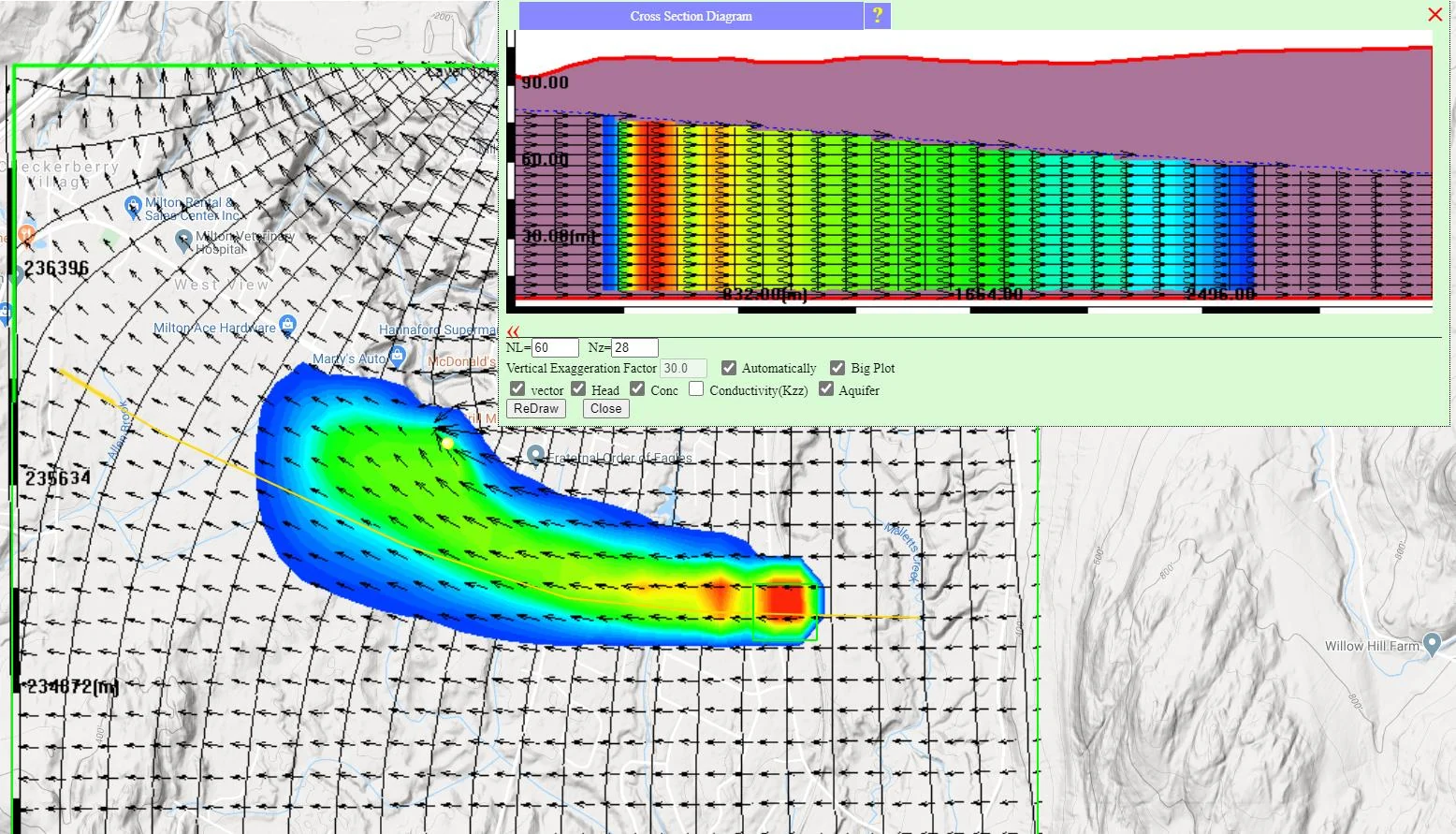
The plume plan view is the most immediate output of transport simulation. What to look for:
- Plume trajectory — does the plume go where flow predicts? Advection should dominate the plume's axis; any deflection usually indicates heterogeneity or source positioning.
- Plume shape — elongated in the flow direction (characteristic of anisotropic dispersion with αL > αT); rounded (isotropic or strong transverse dispersion); complex (heterogeneous aquifer, multiple sources, or boundary interaction).
- Contour spacing — tight contours at the leading edge (sharp front, advection-dominated); broad contours (dispersion-dominated or dual-domain release).
- Multiple plumes from multiple sources — overlapping where sources are close; separated where far apart; merging downgradient into a broader plume.
12.9.2 Cross-sections — vertical structure of the plume
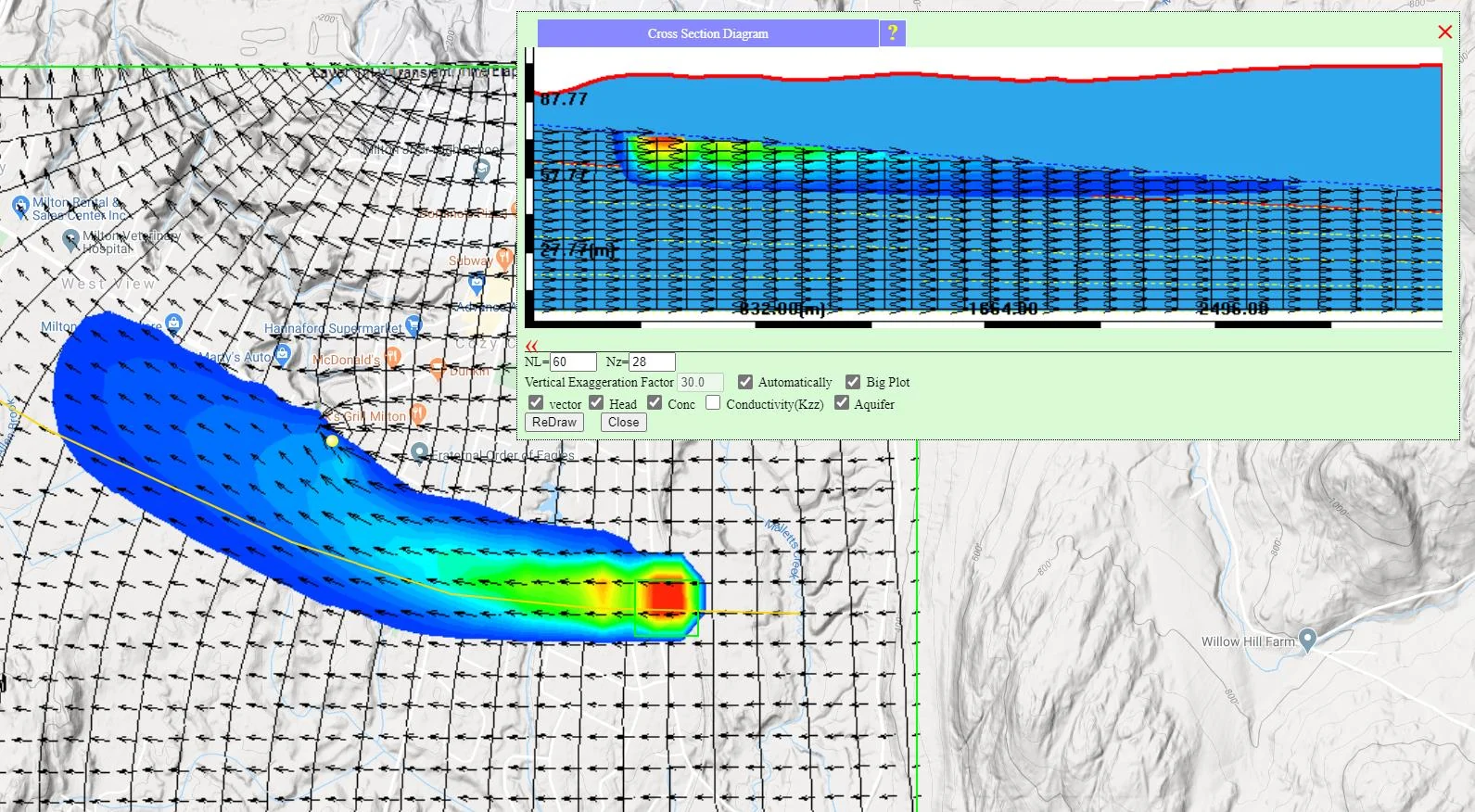
For layered systems and for any plume with vertical structure, cross-sections are essential. Key questions to ask:
- Is the plume staying in the upper aquifer, or migrating downward through confining units?
- If a DNAPL, is the simulation showing the expected vertical descent?
- Are pumping wells capturing the plume, or drawing it deeper?
- For dual-domain or matrix diffusion, is the plume distributing vertically as expected?
12.9.3 Breakthrough curves at monitoring wells
Chapter 9 §9.8.3 introduced breakthrough curves — concentration at a monitoring well plotted against time. They answer quantitative questions that plan views cannot:
- Arrival time — when does concentration first rise above background?
- Time to MCL exceedance — when does concentration exceed the regulatory maximum contaminant level?
- Peak concentration and timing — what is the highest concentration the well sees, and when?
- Decline rate — how fast does concentration fall after the peak?
- Tailing — how long do low-level concentrations persist? Strong tailing suggests dual-domain behavior or slow desorption.
Breakthrough curves are what regulators most often ask for — they are the quantitative summary of risk at a receptor.
12.9.4 Transport mass balance
The water balance from Ch. 8 §8.4 has a transport analog: the mass balance tracks contamination entering, leaving, and accumulating in the domain. Checking it is essential for any serious transport calibration.
Mass inflow categories:
- Internal source release (from source zones)
- Injection well mass input
- Polluted recharge mass input
- Mass inflow through boundaries
Mass outflow categories:
- Mass extracted via pumping wells
- Mass discharged at one-way drains and losing streams
- Mass outflow through boundaries
- First-order decay (mass destroyed, not transported)
- Reaction network consumption (for multi-species simulations)
Storage change:
- Mass in the dissolved phase (mobile plus immobile for dual-domain)
- Mass in the sorbed phase
In a well-constructed steady-state transport simulation, the mass balance closes: inflows = outflows + storage change. Imbalances larger than 1-2% usually indicate convergence issues or configuration problems worth investigating.
12.9.5 A real example — the Mancelona TCE plume
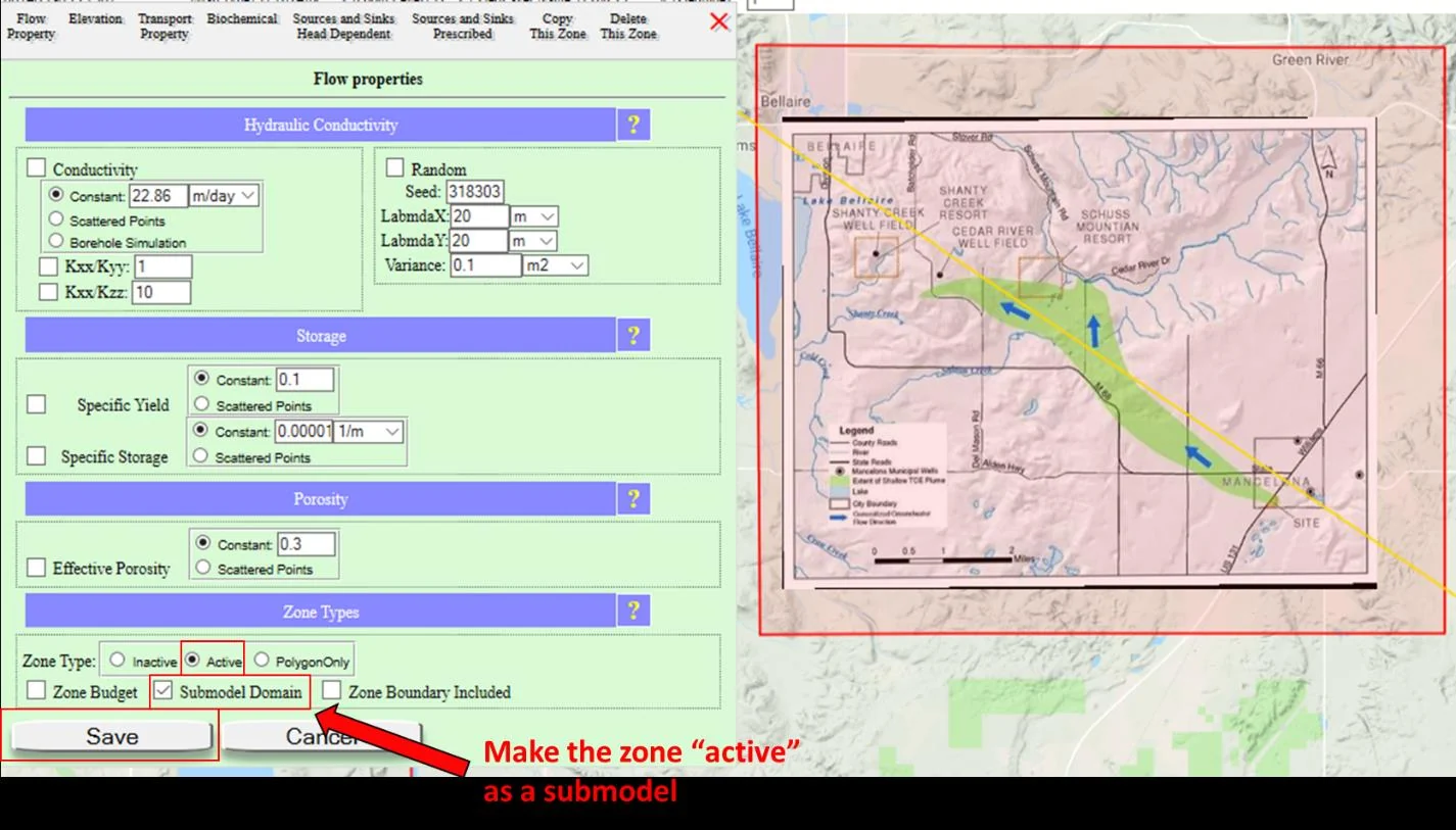
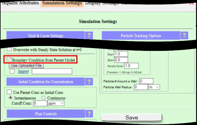
The Mancelona case (northern Michigan) is a real TCE contamination investigation. A historical source area near a former Wickes Manufacturing facility released TCE that migrated for decades through a glacial-outwash aquifer toward local water-supply wells. The case study models TCE as a single species — daughter products were not part of the investigation objectives, so the simulation tracks TCE alone rather than engaging a multi-species reaction module. The workflow is a good example of a focused single-species transport model: regional base model, submodel for the source area with refined grid, single-species TCE transport with sorption and first-order decay, forward particle tracking from the source area to confirm the flow trajectory, and calibration against observed plume concentrations. See the case study documentation for the complete workflow, and §12.6 of this chapter for when multi-species modules are worth engaging.
The flow model and the transport model test each other. If the simulated plume goes where the real plume goes, your flow field is right. If the simulated arrival times and concentrations match observed breakthrough curves, your transport parameters (dispersion, sorption, decay) are right. When both match, you have a defensible model that can be used for prediction — risk assessment, remediation design, regulatory decisions. When they don't match, the mismatch points you to what needs refining. Transport calibration (Ch. 17) is therefore not separate from flow calibration; they constrain each other.
To go deeper
- Chapter 13 — Nested Modeling — next chapter. Nested submodels are the primary remedy for numerical dispersion (§12.4.3) — get fine ijk resolution where transport detail matters without paying for it region-wide.
- Chapter 17 — Calibration — how to calibrate transport parameters against observed plumes and breakthrough curves.
- Chapter 18 — Stochastic Modeling — Monte Carlo transport for probabilistic risk assessment.
- Chapter 9 — Transient Simulation — transport is almost always transient; §9.8 on reading transient results applies directly.
- Case Study: Mancelona TCE Plume — a complete real-world transport simulation with calibration and decisional use.
- Quick Tutorial 5: Contaminant Transport — hands-on walkthrough of a source zone and plume simulation.
- Quick Tutorial 17: Monte Carlo Transport — extending transport into the probabilistic domain.