This end-to-end case study demonstrates how to use IGW-NET to develop, calibrate, and apply a coupled flow-and-transport simulator for the Wickes Manufacturing TCE plume in Mancelona, Michigan — one of the largest groundwater contamination plumes in the United States and the largest TCE plume in Michigan. TCE is a known carcinogen.
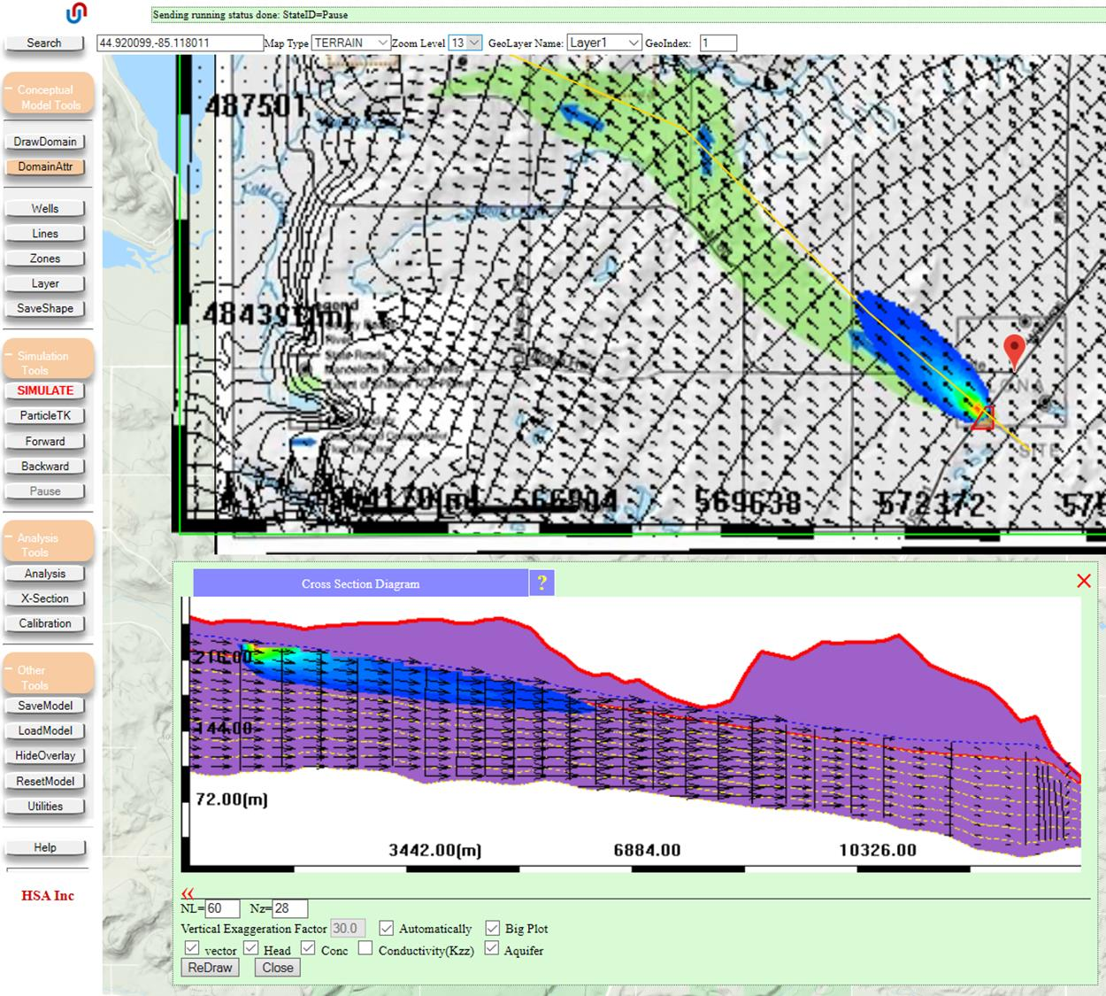
The site's proper treatment demands multi-scale modeling: a large regional domain captures the prevailing flow field and provides boundary conditions to a finer-grid local submodel that resolves plume detail around the source. Once calibrated, the model is used to predict plume migration and design a purge well for active remediation. Finally, vertical computational layers are added to reveal that the plume is not vertically mixed — it occupies primarily the upper third of the aquifer, consistent with a surface-source origin.
The site and the problem
From the 1940s through the 1950s, Wickes Manufacturing operated a plant in Mancelona, Michigan (a small town in the northwestern Lower Peninsula). The plant used chlorinated degreasing solvents — principally trichloroethylene (TCE) — and disposed of waste solvents in shallow pits on site. Over subsequent decades the TCE has migrated northwest through the surficial glacial aquifer, producing a plume that is now one of the largest of its kind in the United States. The plume trends toward a well field that provides drinking water to private residences and nearby municipalities, creating a source-protection problem of direct public-health consequence.
Simulating the plume's transport and planning remediation operations requires detailed flow information at the site, but site-specific flow conditions are influenced by regional flow patterns. The proper approach is nested modeling: a coarser regional model establishes the far-field head distribution and provides boundary conditions to a finer local model that resolves plume-scale detail.
1. Create model domains and overlay the site map
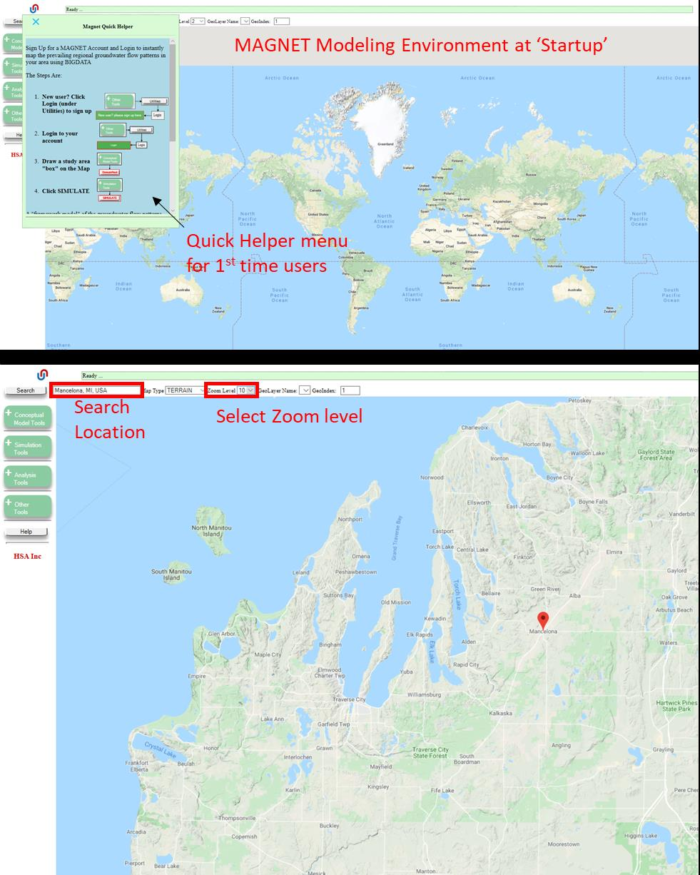
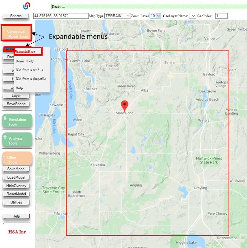
In the IGW-NET modeling environment, after zooming to Mancelona at a regional scale, the DrawDomain → DomainRect tool is used to draw a rectangular regional domain covering the site and surrounding region. Two mouse clicks (one per diagonal corner) are sufficient.
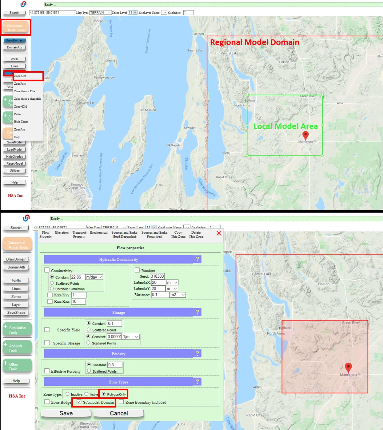
A local submodel zone is then added using ZoneRect, covering Mancelona itself and the area to the northwest. Critically, the zone is initially configured as PolygonOnly in its ZoneAttr Flow Property tab — this flag tells the solver to ignore the zone during the first simulation runs so the regional model can be calibrated independently. After calibration, the zone will be switched to Active.
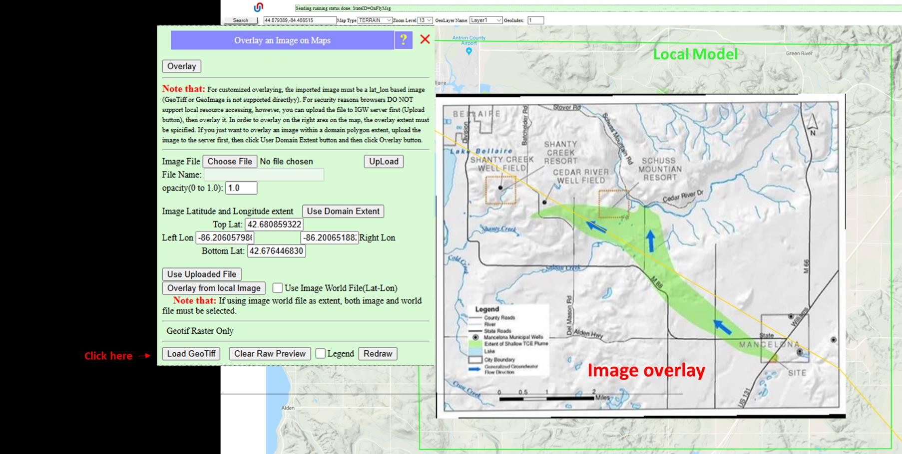
For visual context, a georeferenced plume map is overlaid using Utilities → Overlay myImage. The image shows the previously-delineated TCE plume extent from traditional hydrogeological field methods — a benchmark against which the model results can be compared later.
2. Regional model parameters
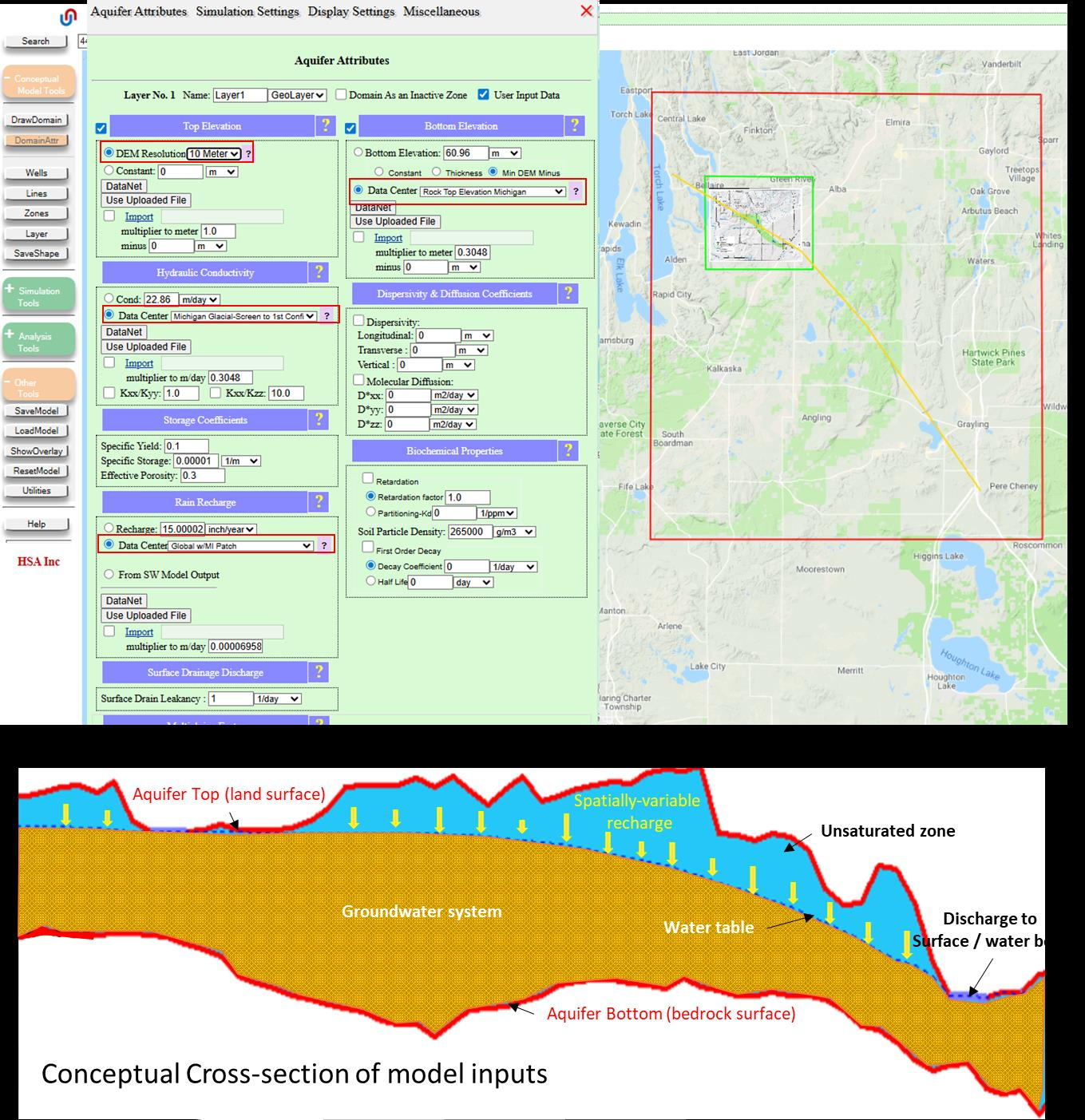
The DomainAttr menu is used to assign aquifer attributes. Every scalar is linked to a MAGNET4WATER Data Center raster layer — spatial variability comes from the server, not from uniform manual input:
- Top elevation: 10 m Digital Elevation Model
- Bottom elevation: Michigan bedrock surface raster (built from well records)
- Hydraulic conductivity: Michigan Glacial-Screen to 1st Confining Unit raster
- Recharge: Global w/MI Patch long-term mean recharge
Cond=22.86 m/day) is a fallback, not the actual value used. The actual values come from the spatially-variable raster — see Fallback vs spatial values for why this matters when someone reviews your model file.
3. Regional simulation
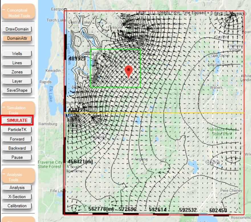
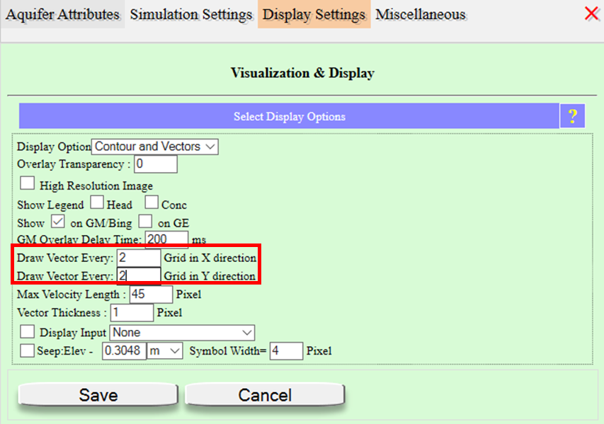
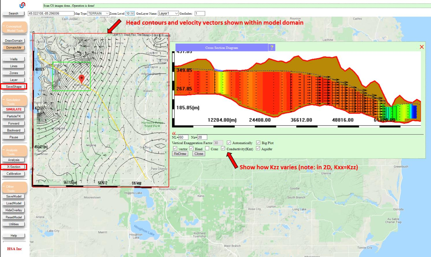
With SIMULATE in steady-state mode, the regional flow field is solved. Head contours and velocity vectors appear over the domain. In highly-gradient areas — near regional discharge features — vector density can make the display crowded; adjusting DomainAttr → Display Settings → Draw Vector Every: 2 grids spaces the vectors for readability.
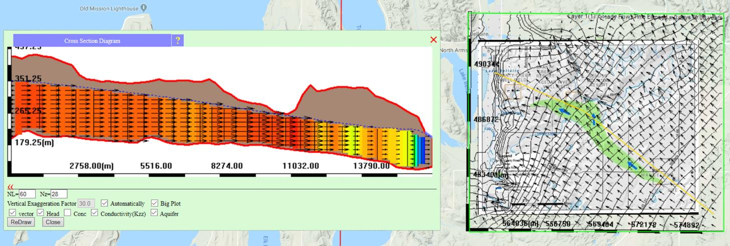
An X-section (cross-section) is drawn from the regional recharge area to the regional discharge area, displaying vertical hydraulic conductivity variability. In this 2D setup, Kxx = Kzz, so the coloring reflects the Data Center raster variability along the section.
4. Evaluate model performance (calibration)
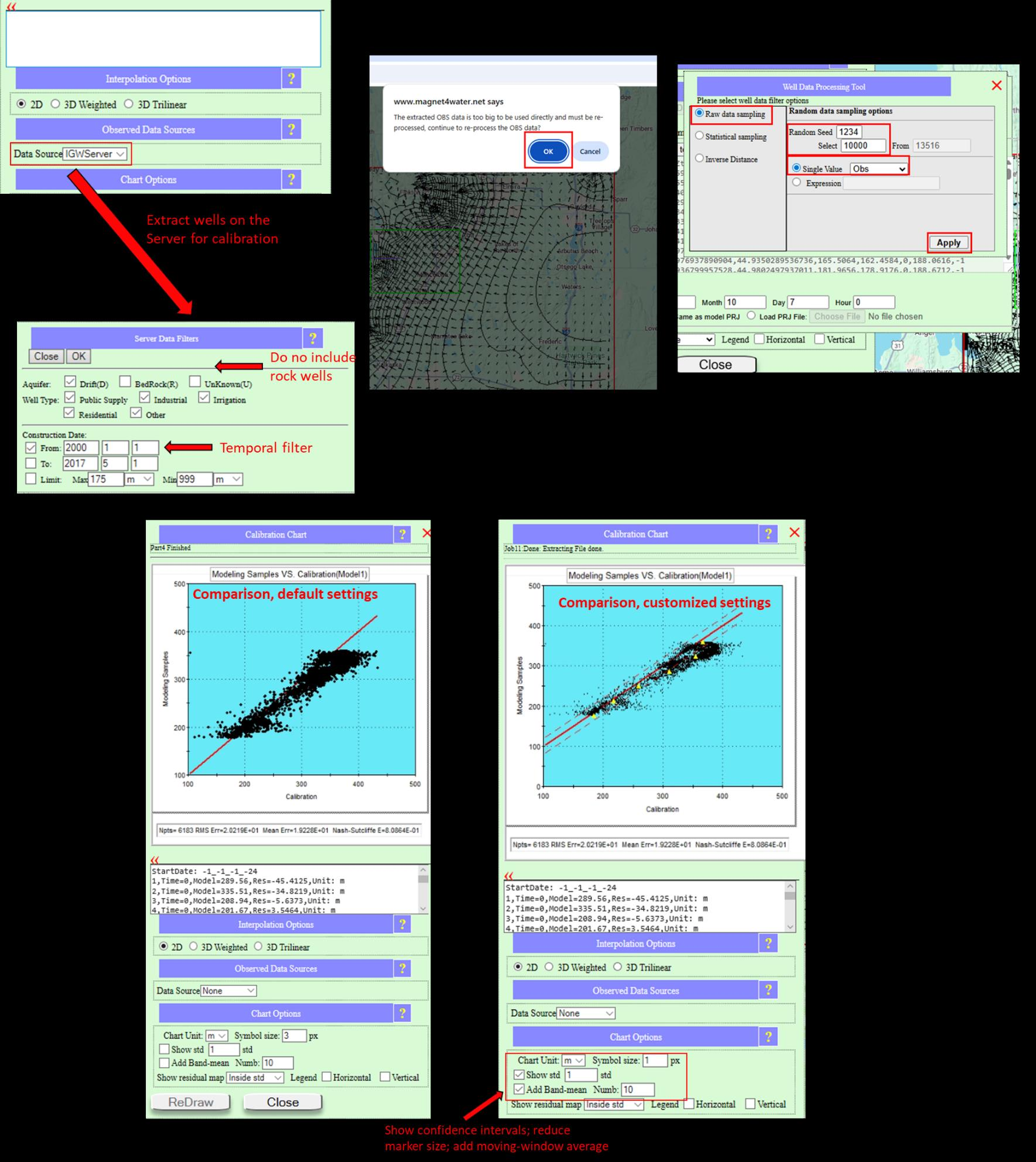
The Calibration tool compares simulated heads against Static Water Levels (SWLs) — measurements of water level taken at the time wells were installed, before any pumping. The data source is set to IGWServer, with filters applied:
- Aquifer type: glacial drift only (no bedrock wells — they respond to different flow regimes)
- Construction date: after 2000 (to avoid old, less reliable records)
The Well Data Processing Tool is used to randomly sample 10,000 SWLs as calibration targets. The chart customization adds a 1σ confidence band, a moving-window (band-mean) average, and reduces marker size for clarity.
5. Adjust K and recharge to improve performance
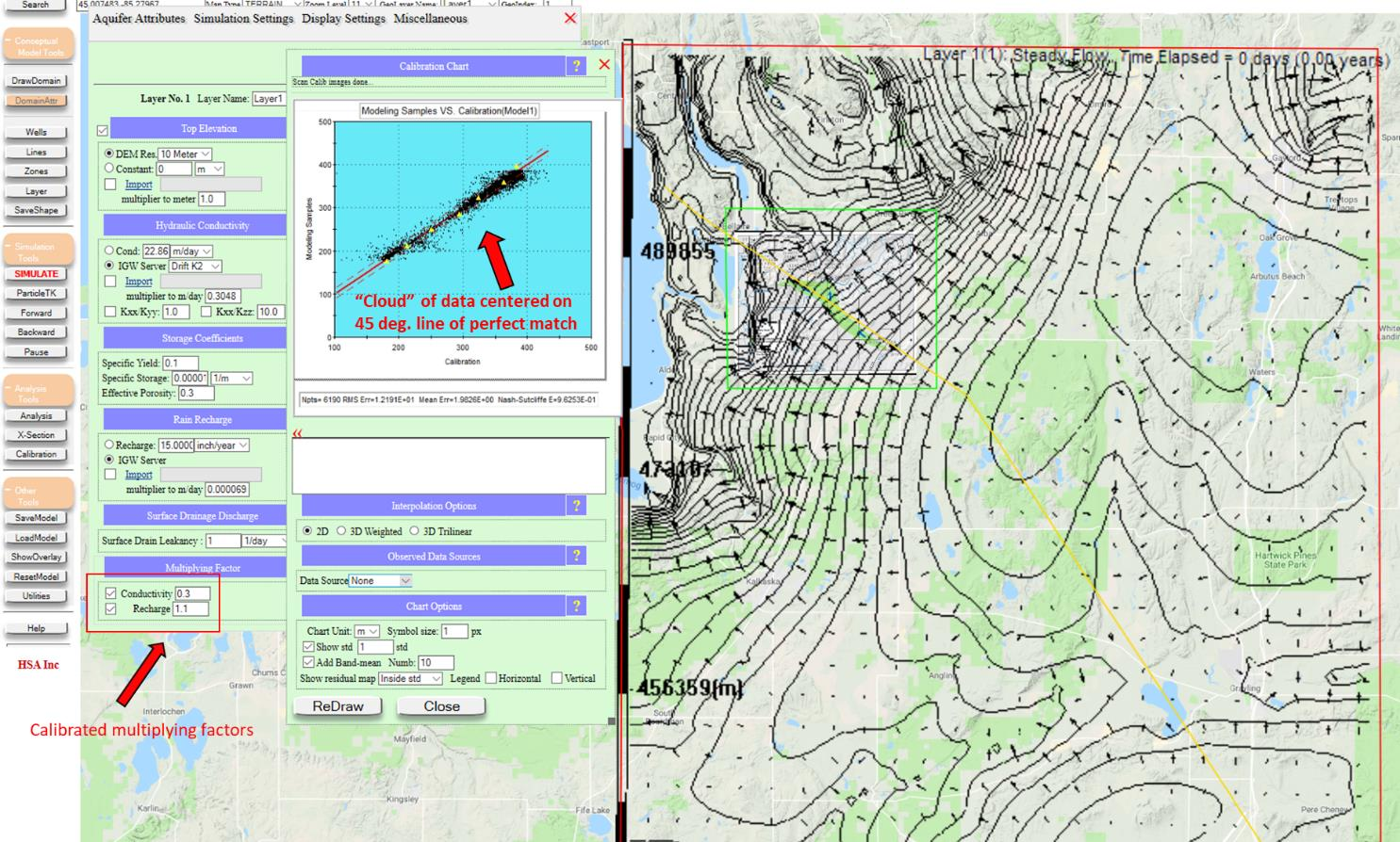
In DomainAttr, domain-wide multipliers are applied: K × 0.3 and Recharge × 1.1. A K multiplier of 0.3 means every cell's hydraulic conductivity from the Data Center raster is reduced by 70%; the recharge multiplier of 1.1 means every cell's recharge is increased by 10%. The resulting calibration cloud and the band-mean are both centered on the 45-degree line of perfect match.
6. Activate the local submodel
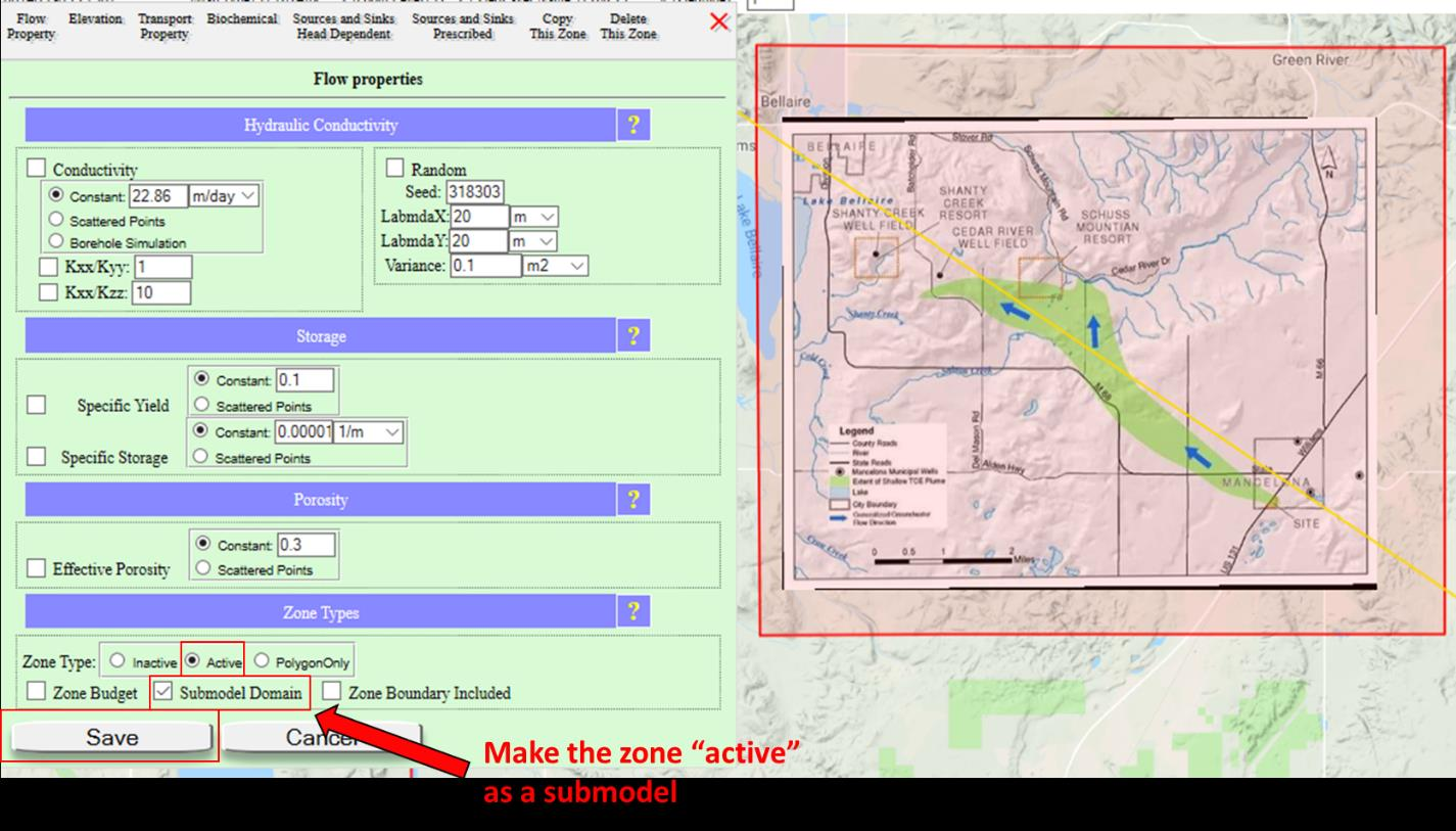
With the regional model calibrated, the local zone is switched from PolygonOnly to Active. Using Utilities → Geometry unlocked, the zone nodes become clickable; clicking any node opens ZoneAttr, where the Flow Property tab is updated: Submodel Domain checked, Zone Type = Active.
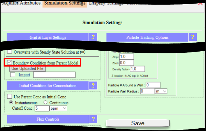
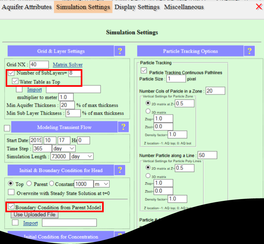
In the Simulation Settings tab of DomainAttr, the Boundary Condition from Parent Model checkbox is turned on. This tells the solver to use the last regional simulation's head solution as the prescribed-head boundary for the local model.
The local model is then simulated, producing a refined head field and a new cross-section showing detailed local flow patterns.
7. Add the Cedar River as a stream feature
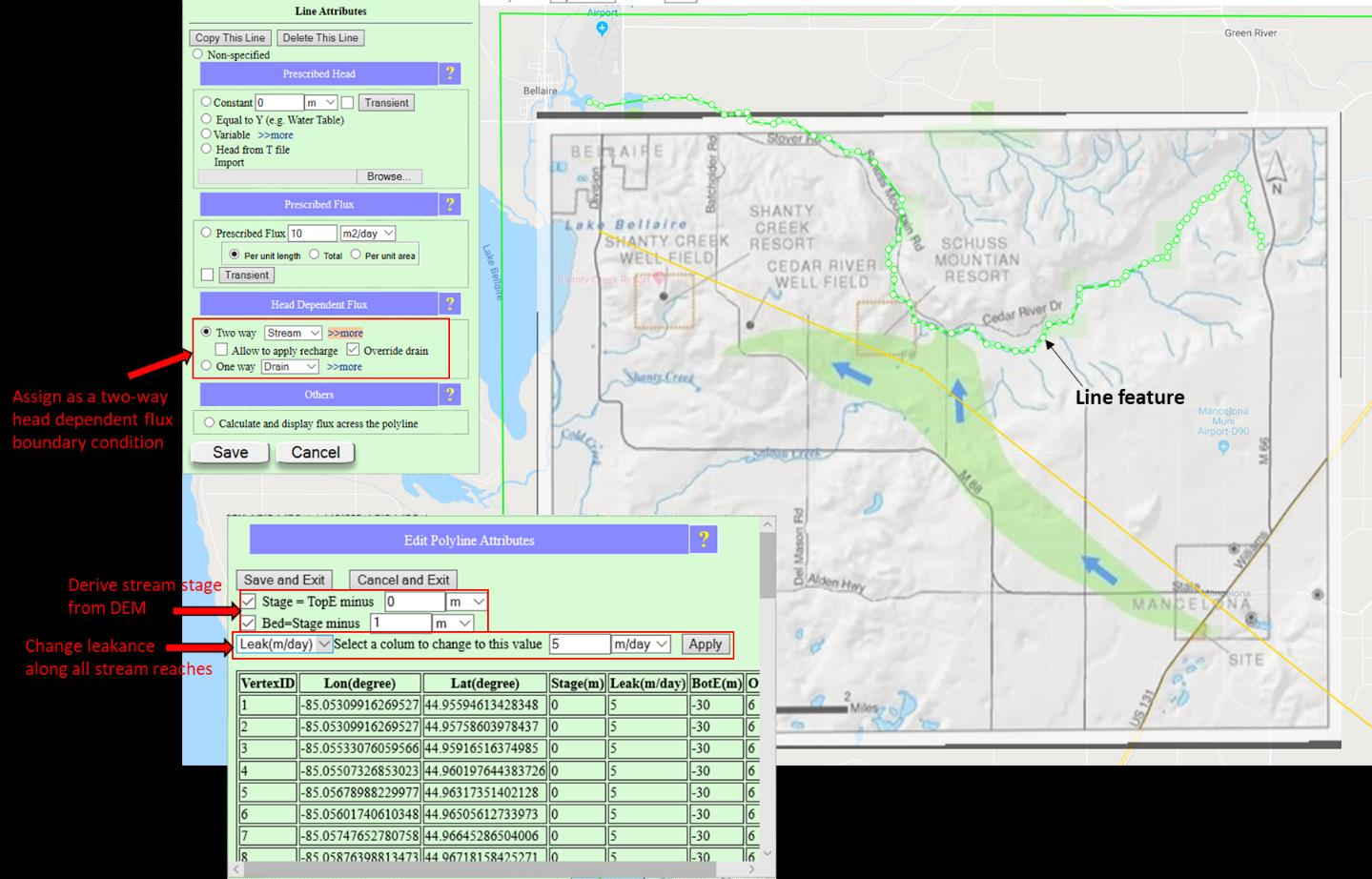
The Cedar River is a salient feature of the site, situated north-northeast of the plume and eventually draining to Lake Bellaire. It is added using DrawLine; click-and-point adds vertices along the river's path. SaveShape finalizes the polyline and opens the Line Attributes menu, where the river is configured as a two-way head-dependent boundary:
- Stream stage: equal to aquifer top (DEM)
- Stream bottom: stage − 1 m
- Leakance: 5 m/day (applied uniformly along all stream reaches)
8. Contamination source and monitoring well
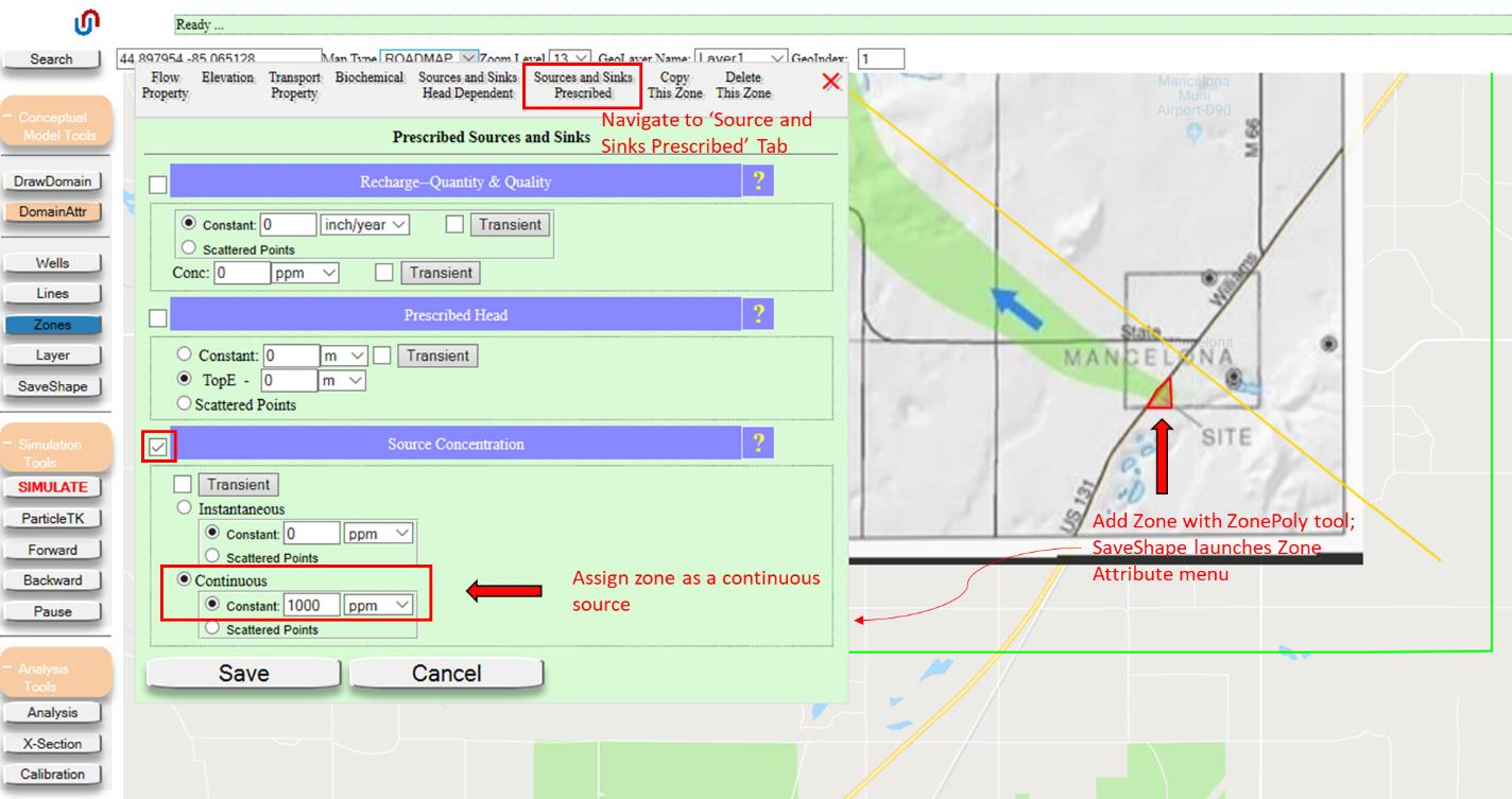
Zooming in to the former Wickes Manufacturing property, a ZonePoly is drawn at the site. In ZoneAttr → Source and Sinks Prescribed, the feature is assigned as a continuous source with concentration 1000 ppm.
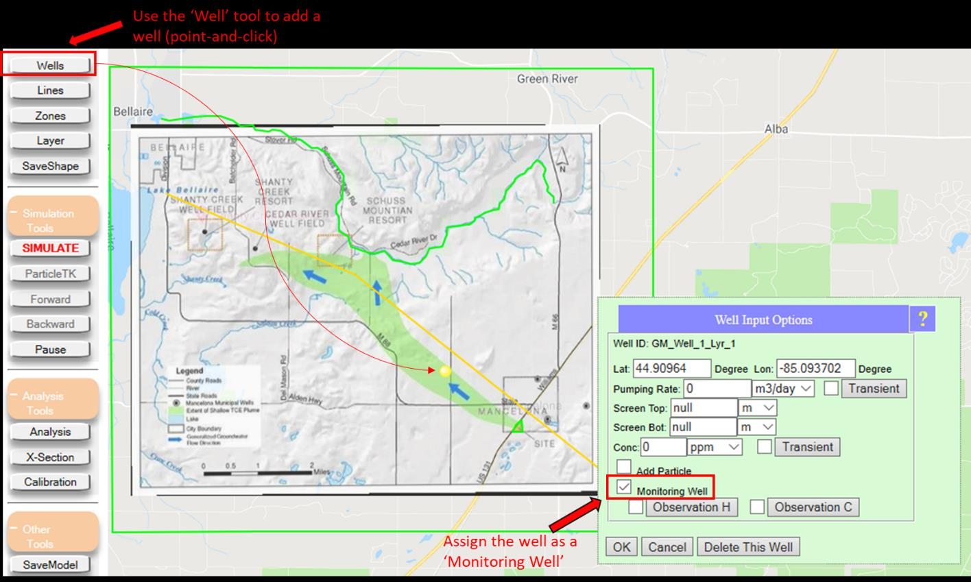
A monitoring well is added downstream with DrawWell, with the Monitoring Well option enabled. This causes IGW-NET to track concentration at that location over time and produce a breakthrough curve.
9. Simulate transport and compare with field delineation
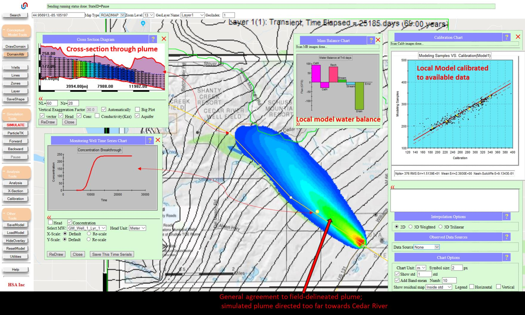
After ensuring Boundary Conditions from Parent Model is still checked (it gets unchecked after each simulation), the local model is submitted. The simulation is steady-state in the flow field but transient in concentration — the plume spreads over time using the fixed flow field. Analysis Tools → Analysis → Display Charts opens the monitoring well breakthrough curve, the cross-section, and the mass balance chart.
DrawWell closes that gap.
10. Design a purge well for remediation
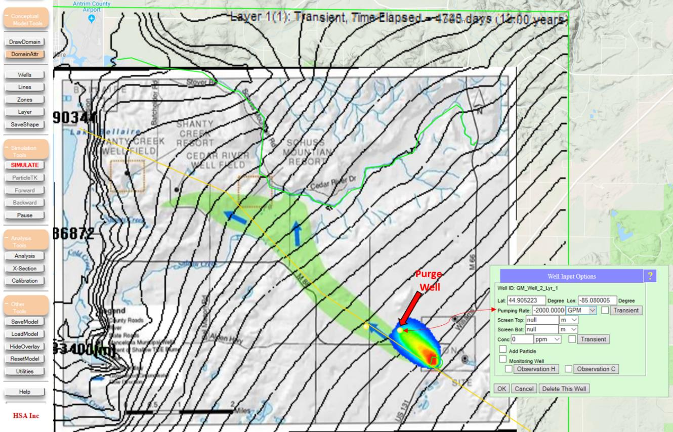
A remediation extraction well is added downstream of the source using DrawWell, with an aggressive pumping rate of −2000 GPM (negative denotes extraction). After resubmitting the simulation with parent-derived boundary conditions, the contour lines bend toward the purge well — the classic signature of capture — and the simulated plume extent contracts dramatically.
11. Add vertical detail — sublayers and a surface source
The 2D simulation so far has assumed the plume is perfectly mixed in the vertical direction. In reality, TCE enters the groundwater system from above via infiltration of recharge through the spill pits. Resolving this requires both vertical computational layers and a surface-source formulation.
Convert the source
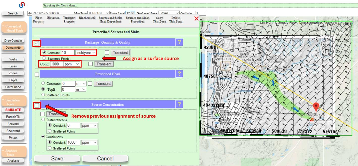
In ZoneAttr → Source and Sinks Prescribed for the spill zone:
- Uncheck Source Concentrations
- Check Recharge−Quantity & Quality
- Enter a constant infiltration rate of 10 inch/year
- Enter source concentration of 1000 ppm
Add computational layers
In DomainAttr → Simulation Settings:
- Check Water Table as Top
- Check Number of SubLayers and set to 8
When the model is re-simulated, the plume now occupies primarily the upper ~1/3 of the aquifer rather than being vertically mixed. This matches reality for surface-sourced dissolved-phase contaminants migrating laterally in a shallow flow system.
Source Provenance
- Original document
- IGW-NET Tutorial: Massive Plume Migration in Northern Michigan Community (PDF)
- Site location
- Mancelona, Michigan, USA — approximately 44.90°N, 85.06°W
- Contaminant
- Trichloroethylene (TCE) — known carcinogen
- Source facility
- Wickes Manufacturing, degreasing solvent disposal (1940s–1950s)
- Platform
- IGW-NET / MAGNET4WATER
- Last reviewed
- 2026-04-20