The quick read — 90 seconds
- Structure first, calibration second. A calibrated model is not necessarily a correct model. If the conceptual structure is wrong (wrong BCs, missing features, wrong layering, wrong aquifer-system framework), calibration will compensate by pushing parameters to unphysical values that fit the observations — the model matches data but fails to predict. IGW-NET's real-time modeling, analysis, and visualization are designed so users spend most of their time building a structurally sound conceptual model; calibration refines a sound model, it doesn't rescue a flawed one.
- Calibration means adjusting parameters so simulated heads match observed heads. Before calibration: reasonable guesses. After calibration: parameters consistent with observed reality. The model becomes defensible by being fit to data — provided the structure was sound to begin with.
- Primary observation type: Static Water Levels (SWLs) — water-table elevations measured at wells, available from regional well databases (Michigan Wellogic, USGS NWIS, Canadian provincial records) through the IGWServer connection. Millions of SWL records exist across North America; IGW-NET gives you access via the Well Data Processing Tool.
- Filter observations ruthlessly. Bad SWLs make bad calibrations. Remove: wells being pumped when measured, wells in the wrong aquifer layer, transcription errors, decades-old records if current conditions differ. Use the Well Data Processing Tool to sample, spatial-filter, and quality-filter before calibrating.
- Primary parameters: the Multiplying Factors. DomainAttr → Aquifer Attributes → Multiplying Factors has checkboxes (K, Recharge, and others) marked "Calib". Each activates a scalar multiplier applied globally to that field. K × 0.3 tightens the aquifer 3.3×; Recharge × 1.1 adds 10% more water. Simple but powerful global adjustments.
- The calibration chart is your primary diagnostic. Scatter plot of observed (x-axis) vs. simulated (y-axis). Well-calibrated = cloud centered on 45° line with symmetric scatter. Bias above/below = parameter adjustments needed. Wide scatter = model doesn't explain observations well.
- Manual calibration loop: try multiplier values → simulate → view chart → adjust → repeat. Useful for building intuition and handling simple cases.
- Automatic Calibration uses UCODE (USGS universal inverse code) for gradient-based parameter estimation. You flag parameters with Calib checkboxes, provide observations, launch Auto-Calibration; UCODE searches for the parameter set that minimizes the objective function (sum of squared residuals). Outputs optimized multipliers plus sensitivity/uncertainty diagnostics.
- K-recharge non-uniqueness: head observations alone cannot separate K from Recharge. The head field depends on K/R, not on K and R individually. To fix the absolute magnitudes, you need additional observations that depend on fluxes — baseflow rates, lake stages, pump test responses.
- Multi-target calibration fits multiple observation types simultaneously — well heads AND lake stages, heads AND baseflow. Essential for coupled models; breaks K-recharge non-uniqueness. The Barron Lake case calibrates against 11 private well SWLs plus observed lake level time series jointly.
- Pitfalls: overfitting with too many parameters; bad observations passed through; claiming K is physical when only K/R is constrained; local minima in auto-cal; systematic residual patterns that signal real model problems; trusting a "perfect" fit.
18.1 What Calibration Is — and What "Calibrated" Means
Every groundwater model makes assumptions about parameters that are not directly measured everywhere in the domain. Calibration is the process of constraining those assumptions with observations, producing a model whose parameters are demonstrably consistent with observed reality rather than just with initial guesses.
18.1.1 Why calibrate
Consider a model at the start of a project. The aquifer K comes from the Data Center default (or from T-PROGS class K values from Ch. 17); the recharge comes from a climate raster; the stream leakance is the IGW-NET default for that stream order (Ch. 14). None of these values were measured at your specific site. They are starting points drawn from typical values and regional defaults — educated guesses that may be off by factors of 2, 5, or 10.
Without calibration, the model's output is an educated guess about the aquifer's behavior, built from educated guesses about the parameters. With calibration, the parameters have been adjusted until the model's simulated heads match observations at specific well locations. The model now has empirical grounding: the parameters are consistent with measured reality at those locations, and by extension (with appropriate caution) at locations between them.
18.1.2 What "calibrated" really means
A calibrated model is not a perfect model. It is a model whose parameters have been adjusted so that simulated values match observations within acceptable tolerance, where the tolerance depends on the question being asked.
- For a regional water-supply assessment, matching heads to within a few meters may be adequate — regional-scale decisions don't depend on local-scale precision.
- For a wellhead protection analysis, local head gradients matter more; tolerance might be tenths of meters.
- For a contaminant transport study, local velocities are critical; tolerance should match the local gradient structure.
- For a coupled lake-aquifer model (Ch. 15), lake stages need to match to within centimeters to constrain the water balance meaningfully.
"Calibrated" is a statement about fit quality relative to the problem's requirements, not a binary yes/no. Two calibrations can both be legitimate: one matching heads to 5 m tolerance for regional work, another matching heads to 0.2 m for a specific well-capture question. Both are calibrated — to different levels of precision, for different purposes.
Before calibrating, ask: what question does this model need to answer, and what tolerance does that question require? Then calibrate to that tolerance. Chasing arbitrary precision — matching every well to within a centimeter — is usually overfitting or wasted effort. Matching only regional averages when local details matter is under-calibration. The right target is set by the problem, not by the calibration algorithm's capabilities.
18.1.3 Structure first, calibration second — why conceptual soundness matters more
A calibrated model is not necessarily a correct model. This is the single most important thing to understand about calibration, and the reason IGW-NET's whole interaction paradigm is designed the way it is.
Here is the failure mode. Suppose the conceptual model is structurally wrong — the layering scheme is inappropriate, a critical stream or lake is missing, the boundary conditions are misplaced, the fundamental framework for the aquifer system doesn't match reality. You run the model; simulated heads don't match observed heads. You turn to calibration. You adjust multipliers; you let UCODE search; eventually you find a parameter set that produces a well-behaved calibration chart with the scatter cloud centered on the 45° line. The RMSE looks good; the bias is gone.
What actually happened: the calibration found parameter values that compensate for the structural flaws. K was pushed unphysically low to make up for a missing constant-head boundary; recharge was inflated to balance a missing lake; leakance was tuned to mask inadequate layering. The parameters no longer represent real aquifer properties — they represent the combined effects of real properties plus structural error. The model fits the calibration data by coincidence of compensating errors.
The consequence: when you use this "calibrated" model for prediction — a new pumping scenario, a future climate condition, a contaminant spill not represented in the calibration observations — the prediction is wrong. The compensating errors that made the calibration fit don't necessarily compensate correctly under the new conditions. The model was fit, not understood; it matched the past, but cannot forecast the future. In the worst cases, a carefully-calibrated structurally-wrong model is more dangerously wrong than an un-calibrated one because the good calibration statistics give false confidence in its predictions.
Calibration refines a structurally sound model; it cannot rescue a structurally flawed one. Parameters tuned to compensate for structural errors match the calibration data by coincidence and fail under prediction. Investing heavily in structural soundness before calibration is not a luxury — it is a prerequisite for a predictive model.
The right order: get the conceptual model right first. Only then calibrate. Time spent on structural understanding pays back multiple times over during calibration and prediction; time spent on calibration before structural understanding is often wasted or worse than wasted.
Why IGW-NET is designed the way it is
IGW-NET's core interaction design — real-time modeling, interactive analysis, instantaneous visualization — is built around this principle. Most of the user's modeling time is intended to be spent building a structurally sound conceptual model, not on parameter-fitting mechanics. The platform supports this by:
- Real-time solution response. Change the layering, change a boundary condition, add a stream, move a zone boundary — and the flow field updates in real time. You see immediately whether the change matters, and in what way. This is conceptual-model iteration at the speed of thought.
- Interactive analysis tools. Cross-sections, particle tracks, water-budget reports, flow-net visualizations — all available inline, not after a batch post-processing step. The modeler can interrogate the model's structural choices rapidly.
- Visualization that reveals structure. Head contours and velocity vectors show where the model is doing what. Anomalies (unexpected flow direction, unphysical head gradients) surface quickly and point back to structural issues that need addressing.
- The Data Center as a structural scaffolding. Authoritative elevation, hydrography, climate, geology, and borehole data is available in a click. Structural choices (where do streams go? what are the layer depths? what's the recharge pattern?) start from defensible Data Center defaults rather than rough guesses.
- Calibration arriving late in the workflow. The calibration tools (Calib checkboxes, Automatic Calibration, UCODE) are part of the standard feature set but are introduced only after the structural tools. The workflow's natural sequence is: build, explore, refine structure; then calibrate.
Contrast this with traditional batch-style modeling workflows, where setting up the model takes days or weeks of file preparation, running it takes hours, and visualization requires separate post-processing tools. In that environment, the temptation is to freeze the structure early (so the files don't have to be rebuilt) and spend most of the project's time on parameter calibration — precisely the workflow that produces well-calibrated, structurally-questionable models. IGW-NET inverts this: real-time interactivity collapses the cost of structural iteration, so structural exploration is cheap and calibration becomes the refinement step it should be.
Throughout the rest of this chapter, this principle is in the background. When §18.9 warns about "systematic residual patterns," what it really means is: residual patterns often signal structural problems that calibration can't fix. When §18.9 warns about "trusting a perfect fit," what it really means is: a perfect fit on a structurally-flawed model is a more dangerous thing than an imperfect fit on a sound one. Structure first; calibration second.
18.1.4 The anatomy of a calibration
Every calibration workflow, whether manual or automatic, has the same structure:
Identify observations
What data does the model need to match? Most often: SWLs from wells. Sometimes also: lake stages, baseflow rates, spring discharges, pump-test drawdowns.
Identify parameters to adjust
Which model inputs will be changed in calibration? Typically the K multiplier and Recharge multiplier (IGW-NET's primary calibration knobs). For multi-zone T-PROGS models (§17.5), the per-zone class K values. For coupled lakes, the lake leakance.
Run the simulation with current parameter values
Produce simulated heads (and other outputs) at the observation locations.
Compute residuals
Residual = simulated − observed at each observation location. Positive residual = model over-predicts; negative = under-predicts.
Evaluate fit quality
Statistics (RMSE, R², mean bias) and visualizations (the calibration chart) show how well the model fits overall, and whether there are systematic patterns in the residuals.
Adjust parameters
Either manually (try a different K multiplier) or automatically (let UCODE search). Go back to step 3. Iterate until fit is acceptable.
The rest of this chapter covers these steps in detail.
18.2 Observations — Static Water Levels and Beyond
Calibration needs observations. The primary observation type for regional groundwater modeling is the Static Water Level (SWL) — a measurement of the water-table elevation at a well when the well is not being pumped. IGW-NET provides access to millions of SWL records through the IGWServer connection, plus support for other observation types for specific needs.
18.2.1 What a Static Water Level is
When a water well is drilled, the driller measures the water level in the newly-completed well — the elevation to which water rises in the well when it is not being pumped. This is the Static Water Level, recorded along with the well's coordinates, depth, screen interval, and lithology log. SWLs are a required reporting element in most jurisdictions; regional databases accumulate them as tens of thousands to millions of records per state or province over decades of well drilling.
For groundwater modeling, SWLs are the most abundant, geographically distributed, and directly comparable type of observation available. They directly measure what the model computes — water-table elevation — at point locations across the domain. A typical regional model might use hundreds to thousands of SWLs scattered across the model domain as the calibration target set.
18.2.2 SWL sources in IGW-NET
The IGWServer connection provides access to regional SWL databases:
- United States — state water-well databases (Michigan Wellogic, similar databases for other covered states in approximately 10 states total) plus USGS NWIS records
- Canada — all provincial databases
- Other regions — users supply SWL data in CSV format with coordinates, elevations, and dates
The same regional databases that provide borehole lithology for T-PROGS (Ch. 17 §17.6) also provide SWLs for calibration. A single data request typically returns both the lithology logs and the SWL measurements for the same wells.
18.2.3 Other observation types
SWLs are primary, but not the only calibration target. Other observation types used in IGW-NET calibration:
| Observation type | What it constrains | Typical source |
|---|---|---|
| Lake stage time series | Lake leakance; absolute-magnitude K (breaks K-R non-uniqueness); lake water balance components | Gauge records, LakeLevel CSVs (like LakeLevel2013.csv in the Barron Lake case) |
| Baseflow / stream discharge | Absolute-magnitude K; stream leakance; recharge rate | USGS stream gauges; baseflow separation from flow records |
| Pump test drawdown | Local K and storage parameters; anisotropy | Site-specific aquifer tests; published regional pump tests |
| Spring discharge | Discharge rate from specific springs; regional flow components | Site measurements; hydrologic monitoring programs |
| Transient head time series | Specific storage and specific yield; seasonal response; stress response | Monitoring well hydrographs; agency water-level networks |
Multi-target calibration (§18.8) uses several of these simultaneously. A coupled lake model calibrates against both SWLs and lake stages; a regional water-budget model might combine SWLs, baseflow, and spring discharge.
18.3 Filtering Observations — The Well Data Processing Tool
Not every SWL is a good calibration observation. Raw databases contain records of varying quality — wells that were being pumped when measured, wells screened in the wrong aquifer layer, transcription errors, historical records that don't reflect current conditions. Uncritical use of raw SWL data produces bad calibrations. The Well Data Processing Tool lets you filter aggressively before calibrating.
18.3.1 The setup dialog
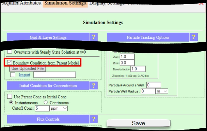
18.3.2 What to filter, and why
Sensible observation filtering removes or adjusts records in these categories:
- Wells being pumped when measured. A pumped well's water level is drawn down and does not represent the static regional water table. Unless the driller's report confirms quiescent conditions, default to excluding clearly-active wells.
- Wells screened in the wrong aquifer layer. In multi-layer models (Ch. 10), a deep well in a confined aquifer should be compared against simulated heads in the appropriate layer, not the unconfined surface layer. Depth filtering ensures each SWL is compared against the right simulated head.
- Very old records. An SWL measured in 1965 may not reflect current conditions if the aquifer has been substantially pumped or climate has shifted. For current-condition modeling, filter to recent records (last 10-20 years, typically). For historical modeling, use date-matched observations.
- Obvious errors. SWLs reported as -99, 0, or the same as the land surface elevation are data-entry problems. Filter out records with implausible values.
- Duplicate or clustered wells. A dense cluster of wells at one location doesn't provide independent calibration information — they all measure the same local head. Random sampling (sampling tool options) or spatial thinning spreads observations across the domain.
- Wells in known-anomalous conditions. Wells near heavy pumping centers, near injection wells, or in specifically-disturbed hydrologic settings may not represent the model's assumed conditions. Exclude these from regional calibration; consider them separately.
18.3.3 The random sampling option
A common filtering approach: from a dense regional database with 50,000+ SWL records, randomly sample 5,000–10,000 for calibration use. This:
- Spreads observations approximately uniformly across the domain
- Avoids over-representing areas with historically heavier drilling
- Keeps the calibration computation tractable (10,000 observations × many parameter sets is manageable; 50,000 × many is slow)
- Provides plenty of observations to constrain modest parameter counts (10,000 observations for 10 parameters is well over the 20% rule of thumb)
The random sample should be reproducible — IGW-NET uses a seed so re-running the same configuration produces the same sample. This lets you iterate the calibration meaningfully.
There's a temptation to filter out SWLs that "disagree" with the model — to keep only observations that the model fits well. This is cheating, not filtering. Legitimate filtering removes observations that are known-bad (pumped wells, wrong layer, errors). Systematic removal of observations the model can't match is systematically biasing the calibration toward whatever the model already says; it doesn't improve the model, it hides the problem.
Use geographic or depth filtering based on a priori information about the well. Don't use residual-magnitude filtering except to spot-check specific outliers that have a non-model-related cause.
18.4 Parameters — The Multipliers
IGW-NET's primary calibration knobs are the Multiplying Factors — scalar adjustments applied globally to specific model fields. This section covers which multipliers exist, where to configure them, and how to activate them for calibration.
18.4.1 What a multiplier is
A multiplier is a global scalar applied to an entire field. K multiplier 0.3 means every K value in the model — whether from a single bulk K, from scattered-point interpolation, from T-PROGS class values, or from T-PROGS zones — is multiplied by 0.3. The spatial pattern is preserved; only the absolute magnitude changes.
Multipliers are chosen rather than per-cell parameters because:
- Parametric simplicity. One multiplier per field means few calibration parameters. A model with K multiplier and Recharge multiplier calibrated has 2 parameters; calibrating every cell's K independently would be thousands of parameters. The multiplier approach is tractable; the per-cell approach is almost always under-constrained.
- The spatial pattern is often known better than the magnitude. T-PROGS gives you the relative K distribution; Data Center recharge gives you the spatial recharge pattern; what's uncertain is the overall magnitude. A global multiplier captures exactly that.
- Calibration uniqueness. Fewer parameters means more identifiable parameters. Each multiplier can be well-constrained by the calibration data.
18.4.2 The standard multipliers
IGW-NET's primary multipliers, configured in DomainAttr → Aquifer Attributes → Multiplying Factors:
| Multiplier | What it scales | Typical calibration range |
|---|---|---|
| K multiplier | Hydraulic conductivity field (bulk K, scattered-point K, T-PROGS class K values — everywhere K is specified) | 0.1 to 10 (factor of 100 spread); values outside this range suggest the base K is substantially wrong |
| Recharge multiplier | Groundwater recharge rate (uniform value or raster from Data Center) | 0.5 to 2 (factor of 4 spread); recharge is better-constrained by climate data so large adjustments are suspicious |
| Surface Drain Leakancy multiplier | The Level-1 DEM-drain leakance (Ch. 5 §5.8, Ch. 14 §14.2.1) | 0.1 to 10; adjusts how easily aquifer drains to the land surface |
| Stream / Lake leakance multipliers | Level-2 explicit feature leakances (for models with drawn streams and lakes) | 0.1 to 10; adjusts SW-GW exchange strength |
18.4.3 Activating multipliers with Calib checkboxes
Each multiplier has an associated Calib checkbox in the Multiplying Factors section. Checking the box flags that parameter as one the user wants to calibrate:
- Calib checked, manual workflow: You adjust the multiplier value yourself, simulate, view the calibration chart, iterate. The checkbox marks it as a "calibration parameter" for reporting but doesn't automatically vary it.
- Calib checked, Automatic Calibration workflow: UCODE varies this multiplier as part of the parameter search. All Calib-checked multipliers are jointly optimized; unchecked multipliers stay at their current values.
- Calib unchecked: The multiplier keeps its current value (typically 1.0) and is not varied by Automatic Calibration. Use for parameters you want to fix.
For most groundwater modeling, start by calibrating just the K multiplier and Recharge multiplier. Two parameters are easy to understand, easy to calibrate, and capture the dominant magnitude uncertainty in most models. Only add more calibration parameters (leakances, per-zone K) when the two-parameter calibration demonstrably can't fit the observations and you have evidence that the additional parameters are constrained by the data.
Adding parameters doesn't improve calibration quality; it just spreads the fit error around differently. Each new parameter needs supporting observations to be justified.
18.5 The Calibration Chart — Reading Observed vs. Simulated
The calibration chart is the primary visual diagnostic for calibration work. A scatter plot of observed versus simulated values, it shows immediately whether the model fits the data and, if not, in what systematic ways it's off.
18.5.1 Reading the chart
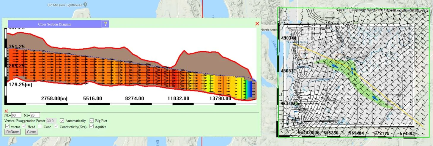
18.5.2 What the chart patterns mean
| Pattern | Interpretation | Typical fix |
|---|---|---|
| Scatter cloud centered on 45° line with moderate spread | Well-calibrated model; parameters are correct on average | No adjustment needed |
| Cloud shifted above 45° line | Model over-predicts heads; water is accumulating in the model more than observed | Increase K multiplier (lets water flow out more easily) OR decrease Recharge multiplier (less water entering) |
| Cloud shifted below 45° line | Model under-predicts heads; water is draining too readily | Decrease K multiplier OR increase Recharge multiplier |
| Tight scatter (low spread around the cloud) | Model explains the observation-to-observation variability well; head field structure is correct | Good sign |
| Wide scatter (high spread) | Model doesn't explain the observation-to-observation variability; head field structure is off, or observations have errors | Investigate: observation quality? Spatial patterns in residuals? Unmodeled heterogeneity? |
| Curved or tilted cloud shape | Non-linear mismatch; the model systematically deviates from the 1:1 line at high and low head values | Often a sign of wrong K at one end of the spectrum, or wrong boundary conditions affecting one region |
| Bimodal or clustered cloud | Different well populations being fit differently; possibly a regional difference the single-zone model can't capture | Consider regional zonation (Ch. 17 §17.5); investigate whether clusters correspond to geologic boundaries |
18.5.3 After calibration
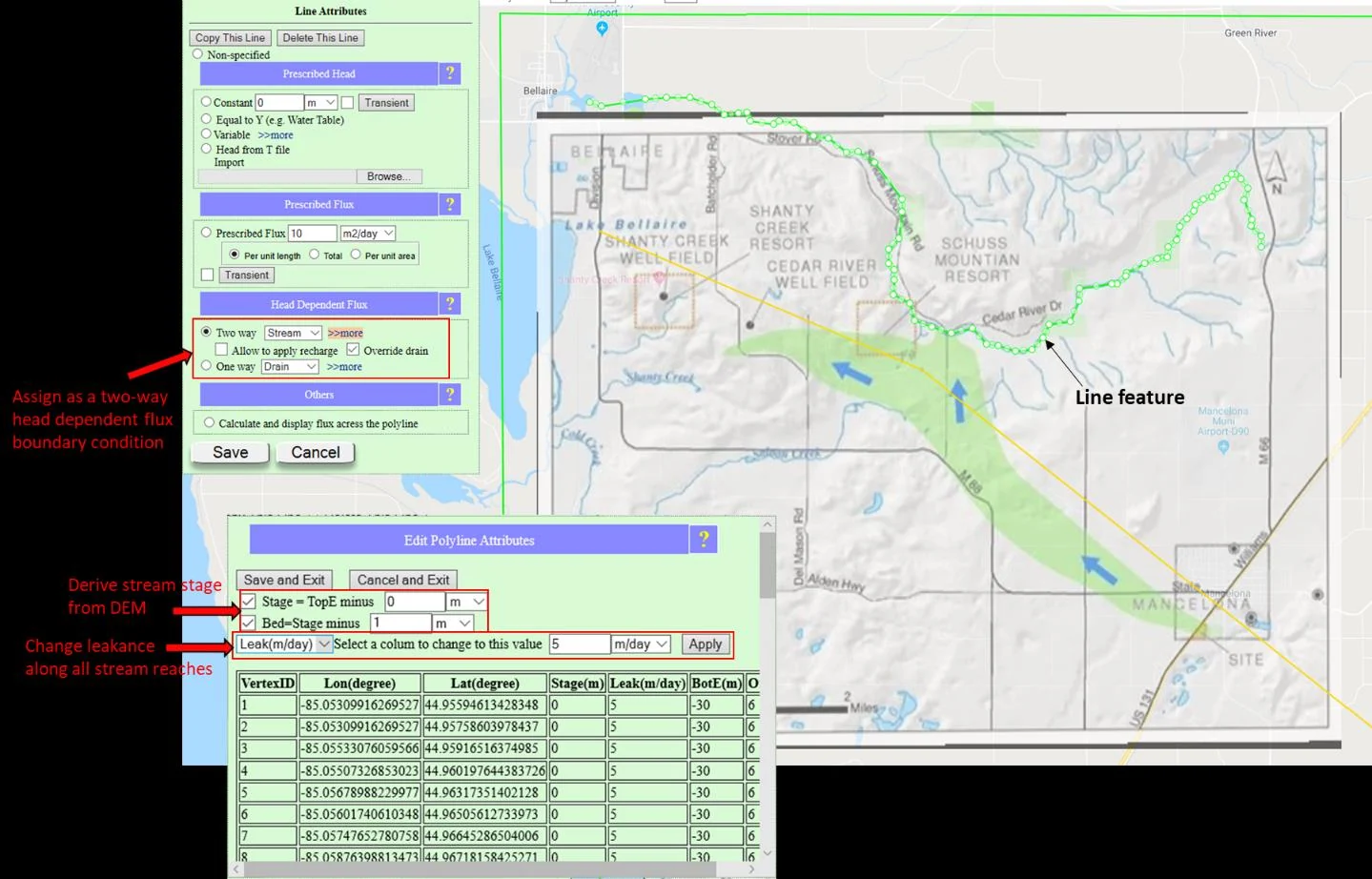
18.5.4 Summary statistics
In addition to the visual chart, IGW-NET reports summary statistics:
- RMSE (Root Mean Square Error) — the square root of the mean squared residual; a single-number summary of fit quality. Lower is better; report what "good" means for your problem's scale.
- Mean bias — mean(simulated − observed). Zero bias means no systematic over- or under-prediction; non-zero bias signals the cloud is off the 45° line.
- R² — fraction of observation variance explained by the model. High R² means the model captures the observation-to-observation variability; low R² means it doesn't.
- Observation count — how many observations contributed to the statistics. More observations = more trustworthy statistics.
18.6 The Manual Calibration Loop
Manual calibration is the traditional approach — the modeler adjusts parameters, simulates, evaluates the chart, iterates. It's slower than Automatic Calibration but builds intuition and handles cases that automated tools don't handle well. For many projects, a round of manual calibration before switching to Automatic is the right sequence.
18.6.1 The loop structure
Start with defaults
Initial K multiplier = 1.0, Recharge multiplier = 1.0. Run the simulation; view the calibration chart.
Observe the systematic bias
Is the cloud above or below the 45° line? How far? Use §18.5.2 to identify the likely parameter adjustment.
Make a substantial adjustment
Don't nudge multipliers by 5%; the signal is usually weaker than the effect. Try K multiplier 0.5 or 2.0, Recharge multiplier 1.5 or 0.7. Re-simulate.
Re-evaluate and refine
Did the bias go down? If yes, you went in the right direction. If the bias reversed (now below the line instead of above), you overshot. Back off halfway. Re-simulate.
Iterate to convergence
Usually 3–8 iterations get you to a visually-unbiased calibration chart. Further refinement is diminishing returns.
Check residual patterns
A calibrated chart shows the cloud centered on 45°, but does the residual pattern on the map make sense? Systematic spatial patterns in residuals indicate real model issues that multiplier adjustments can't fix. Investigate.
18.6.2 When manual calibration is enough
For simple models with 1–3 calibration parameters and well-behaved observations, manual calibration is efficient and adequate. Cases:
- Regional flow models with K and Recharge multipliers
- First-pass calibration of a new model (get to "approximately right" before Automatic Calibration refines)
- Models where the modeler has strong physical intuition and wants to see how parameter changes affect the solution
18.6.3 When to escalate to Automatic
Move to Automatic Calibration (§18.7) when:
- More than 3–4 parameters are being adjusted jointly — manual search becomes combinatorially painful
- Parameter interactions are strong and non-intuitive
- You need formal uncertainty estimates (UCODE produces parameter standard errors)
- You want to use the parameter estimation output as input to stochastic analysis (Ch. 19)
18.7 Automatic Calibration — UCODE Parameter Estimation
Automatic Calibration uses UCODE (USGS Universal inverse COde) to search for the parameter set that minimizes the objective function — the sum of squared residuals between simulated and observed values. The Automatic Calibration tool wraps UCODE in an IGW-NET workflow so the modeler doesn't have to manage UCODE input files directly.
18.7.1 What UCODE does
UCODE is the USGS-supported universal inverse code for parameter estimation in environmental models. Given:
- A forward model that takes parameters as input and produces simulated values (IGW-NET's groundwater solve)
- A set of observations at specific locations
- A list of parameters to estimate (the Calib-checked multipliers and any per-zone K values)
UCODE runs many forward simulations, each with slightly different parameter values, computing how the simulated-observed residuals change with each parameter. Using gradient information, it iteratively searches for the parameter set that produces the smallest total residual sum (the objective function).
18.7.2 The IGW-NET Automatic Calibration workflow
Check Calib boxes for the parameters to calibrate
DomainAttr → Aquifer Attributes → Multiplying Factors → check K, Recharge, and/or other multipliers. UCODE will vary the checked ones.
Set up observations via Well Data Processing Tool
Filter SWLs as described in §18.3. Confirm the observation set is in place before launching calibration.
Launch Automatic Calibration
Via the Automatic Calibration tool in the Simulation Tools area (may be under a specific button or menu option depending on your IGW-NET version — typically labeled "Automatic Calibration" or "Auto-Cal"). Provide initial parameter values and expected ranges.
UCODE runs iterations
Each iteration is a forward simulation plus gradient computation. Typical runs take 10-50 iterations depending on parameter count and observation count. Progress is displayed.
Review the results
UCODE outputs: optimized parameter values, parameter standard errors (uncertainty), parameter correlations, and residual statistics. Also, the calibrated calibration chart (the one you'd see with the optimized parameters).
Accept, reject, or refine
If the optimized parameters are physically reasonable and the fit is acceptable, accept them as the new model defaults. If parameters hit arbitrary bounds or look unphysical (K multiplier = 100), investigate — you may have a non-uniqueness issue or a bad observation. Possibly re-run with different starting points or constrained bounds.
18.7.3 What UCODE gives you beyond parameter values
The key diagnostics UCODE produces, beyond the optimized parameters themselves:
- Parameter standard errors. Uncertainty estimate for each calibrated parameter. A K multiplier of 0.3 ± 0.05 is tightly constrained; 0.3 ± 0.5 is barely constrained. The standard errors tell you which parameters the data really pins down.
- Parameter correlations. Pairwise correlations between calibrated parameters. High correlation (> 0.9 or < −0.9) means the two parameters can't be separated by the data — the classic case is K multiplier and Recharge multiplier, which are typically strongly correlated when only head observations are used (K-recharge non-uniqueness, §18.8).
- Parameter sensitivity. How much the objective function changes per unit change in each parameter. Low sensitivity = the parameter doesn't affect the fit much = data doesn't constrain it well.
- Observation residuals. Per-observation residuals at the optimized parameter values. Large residuals at specific wells flag observations that the calibrated model can't match — investigate whether the observation is bad or the model is missing local structure.
Manual calibration gives you "parameters that make the chart look good." Automatic Calibration gives you parameters plus the whole inverse problem structure: which parameters are well-constrained, which are not, which are correlated, which observations are fit well, which are not. This is substantially richer information and often reveals that the fit obtained manually was only one of many possible fits. When you move from manual to automatic, you gain not just better parameter values but better understanding of the calibration problem itself.
18.8 Multi-Target Calibration — Fitting Multiple Observation Types
A single observation type (usually head SWLs) often can't fully constrain the model. Head observations suffer from K-recharge non-uniqueness; lake stages or baseflow add the flux-based information needed to separate them. Multi-target calibration fits multiple observation types simultaneously, producing more identifiable and trustworthy parameters.
18.8.1 K-recharge non-uniqueness — the canonical case
A steady-state groundwater flow equation is linear in the K/R ratio. Given a fixed spatial pattern of K and R, scaling both by the same factor α produces identical head fields: if (K, R) produces head h(x), then (αK, αR) produces exactly the same h(x). Head observations alone cannot distinguish them.
Consequence: you can "calibrate" a model against SWLs and match them perfectly with K multiplier 0.3 and Recharge multiplier 1.0, OR with K multiplier 0.6 and Recharge multiplier 2.0, OR with K multiplier 0.15 and Recharge multiplier 0.5. All three fit heads equally well; they differ in how much water is actually moving through the aquifer, which is exactly what you usually want to know.
A model calibrated only against head SWLs, with K and Recharge multipliers both active, has arbitrary absolute magnitudes — you've pinned down K/R but not K or R individually. The model will fit heads, but its predictions of: (1) stream baseflow, (2) well yields, (3) time to contamination, (4) lake water balance, (5) any flux-based quantity, will be wrong by whatever factor α actually is. Always add at least one flux-based observation (baseflow, lake stage, pump test) before claiming a calibrated model in absolute terms.
18.8.2 How lake stages break non-uniqueness
In a coupled lake model (Ch. 15), lake stage is governed by the lake's water balance:
dV_lake/dt = Ins − Outs
The Ins and Outs include GW-to-lake flux (gaining cells) and lake-to-GW flux (losing cells), each computed as leakance × (h_lake − h_aq). These fluxes depend on absolute heads and K values, not just the K/R ratio. Matching observed lake stage fixes the absolute magnitudes.
Specifically: if the model has too-low K, the lake-aquifer exchange is too slow, and observed lake stage dynamics (drawdown response, recharge response) are not reproduced — regardless of how well heads match. Lake stage observations provide a flux-based constraint that cannot be satisfied by arbitrary K/R scaling.
18.8.3 The Barron Lake multi-target calibration
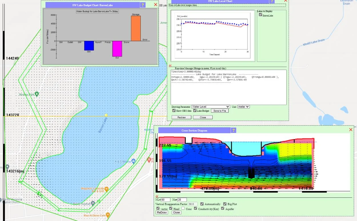
The Barron Lake case study (Ch. 15 §15.4) is a canonical multi-target calibration:
- Observation type 1: 11 private well SWLs. Constrain the spatial distribution of aquifer heads; establish the head pattern and hydraulic gradient directions.
- Observation type 2: Observed lake stage time series (LakeLevel2013.csv, 135-day record). Constrain the lake water balance; fix the absolute magnitudes of K, lake leakance, and recharge.
Without the lake stage observations, the 11-well calibration would be non-unique — many (K, Recharge) combinations would fit. Adding the lake stage pins down the absolute scale; the resulting calibrated model is trustworthy for both well-drawdown predictions and lake-level predictions.
18.8.4 Multi-target weighting
When combining observation types, the calibration objective function weights them:
Objective = w_heads × Σ(h_sim − h_obs)² + w_stage × Σ(stage_sim − stage_obs)²
The weights (w_heads, w_stage) balance how much each observation type matters. Standard practice: weight by the inverse of observation variance — observations with smaller expected errors get more weight. Or: weight to equalize the contribution of each observation type to the objective function, so 10 lake-stage observations don't get drowned out by 500 head observations.
UCODE in IGW-NET handles the weighting automatically based on observation-type defaults; advanced users can override weights per observation if specific observations are known to be especially reliable or unreliable.
18.9 Common Pitfalls
Calibration has failure modes that look like success — charts that look calibrated but aren't, parameter values that seem physical but aren't identifiable, fits that are "too good." This section collects the traps that repeatedly catch modelers.
18.9.1 Overfitting
If you calibrate N parameters with M observations, you need M much larger than N for the calibration to be well-posed. Rule of thumb: M ≥ 5–10 × N, and preferably more. Calibrating 15 parameters with 20 observations gives you 20 equations in 15 unknowns plus noise — effectively fitting the noise, and the "best" parameter set is arbitrary among many that fit equally well.
- Parameter values at arbitrary-looking bounds (K multiplier exactly at 10.0 or 0.1)
- Very high parameter correlations in UCODE output (>0.95)
- Very low parameter sensitivities (parameter doesn't affect the objective much)
- Running UCODE twice from different starting points gives very different parameter values
- Residuals fit exactly at every observation (zero scatter) — if this happens, the calibration is over-specified
Fix: reduce the number of calibration parameters. Accept that some are unidentifiable with available data. Bring in additional observation types before adding more parameters.
18.9.2 Bad observations passed through
If your observation set contains many bad records (pumped wells, wrong-layer, errors), the calibration tries to fit them anyway. The result: parameters that fit bad data. The apparent calibration quality looks fine, but the parameters are wrong.
Signs: unusually high scatter on the calibration chart, systematic residual patterns that don't match any plausible geologic or hydrologic feature, parameter values that conflict with literature expectations. Fix: revisit the observation filtering (§18.3), apply stricter quality criteria, re-calibrate.
18.9.3 K-recharge non-uniqueness hidden as "calibrated"
Already covered in §18.8.1. A model calibrated with head observations only and both K and Recharge multipliers active is not a fully-calibrated model — only K/R is fixed. Claiming specific K values from such a calibration is misleading. Always add flux-based observations before publishing absolute K values.
18.9.4 Local minima in Automatic Calibration
UCODE finds a local minimum of the objective function — possibly not the global minimum. If the objective function is non-convex (has multiple basins), the starting parameter values determine which basin you end up in.
Fix: run Automatic Calibration from several different starting points (K multiplier = 0.3, 1.0, 3.0, etc.) and compare results. If they all converge to the same parameter values, you've likely found the global minimum. If they converge to very different values, the problem is non-unique or has multiple local minima and you need more data to disambiguate.
18.9.5 Systematic residual patterns
A calibration chart centered on 45° is necessary but not sufficient. Check residual patterns spatially:
- Plot residuals on the model map. Are they spatially random, or do wells in one region cluster to positive residuals and wells in another to negative?
- Systematic regional bias indicates the model is missing something in that region — unmodeled recharge variation, a geologic boundary the single-zone model doesn't capture, boundary condition issues, or unrepresented pumping.
- The multiplier adjustment that fixes the aggregate bias doesn't fix the regional pattern; that requires either Ch. 17 regional zonation, different BCs, or better representation of whatever is regionally different.
More broadly: systematic residual patterns are usually the signature of structural problems the calibration can't fix with parameter tuning. When you see a residual pattern, revisit §18.1.3 — parameters can compensate for structural errors in an average sense, but the compensation is spatially imperfect and the residual pattern is the visible leftover. Going back to improve the conceptual model is almost always the right response.
18.9.6 Trusting a perfect fit
A calibration chart where all observations fall exactly on the 45° line (zero scatter) should make you suspicious. Real SWL observations have measurement uncertainty of 0.3–1 m (driller-reported), plus the real aquifer has heterogeneity that a model can't capture perfectly. Zero scatter means either (a) very few observations (trivially fit any way), (b) observations that are actually model-produced or trivially consistent, or (c) over-fitting.
Good calibrations have 1–3 m RMSE for regional models, some residual scatter, and a few outliers that the model can't quite match. That looks realistic. Zero-scatter fits look suspiciously clean; investigate. Remember from §18.1.3: a "perfect fit" on a structurally-flawed model is a more dangerous thing than an imperfect fit on a sound one — the good calibration statistics give false confidence in predictions that may still be very wrong.
18.9.7 Calibration without model-purpose awareness
Calibrating to the tightest possible RMSE regardless of purpose is a trap. A model calibrated to match heads within 0.1 m everywhere may still be wrong for transport predictions if the velocity field is not properly constrained. A regional water-supply model calibrated to match specific well hydrographs may be over-specified for the regional-averaging question it's meant to answer.
Always revisit §18.1.2: what question is this model answering, what tolerance does it require? Calibrate to the answer's needs, not to an abstract "best fit" target.
18.9.8 Calibrating before structural soundness
This is the meta-pitfall that subsumes several of the others (§18.9.3, §18.9.5, §18.9.6). The pattern: jump to calibration while the conceptual model still has unresolved structural issues — layering not fully worked out, boundary conditions not yet defensible, features not yet at the right resolution, zones not yet aligned with geology. Calibration "succeeds" because multipliers absorb the structural errors; you get a calibrated-looking model. Then a new scenario, a new stress, or a new observation exposes that the model was never structurally correct, and all the calibration effort has to be redone.
The signature symptoms: calibrated parameters that drift far from physically-reasonable values (K multiplier > 5 or < 0.1 for an aquifer whose literature values are around 1); parameters that swing widely between successive calibration runs as you add or remove observations; residuals with obvious spatial structure; calibration that "works" for one scenario but fails when evaluated on any other data.
The fix: go back to conceptual modeling. Use IGW-NET's real-time interactivity to try different structural configurations; use visualization to build intuition about what the aquifer is actually doing; confirm the structure is defensible on hydrogeologic grounds before letting UCODE search for parameter values. The time investment in conceptual soundness pays back multiple times during calibration and prediction. This is the entire reason IGW-NET is designed around real-time interaction (§18.1.3) — to make conceptual-model iteration cheap, so the structure is right before calibration is asked to do things it can't.
To go deeper
- Chapter 17 §17.5 — Regional zonation — per-zone class K values as additional calibration parameters; when systematic residual patterns warrant zonation.
- Chapter 15 §15.4 — Barron Lake case study — the canonical multi-target calibration with lake stages + well heads jointly.
- Chapter 19 — Stochastic Modeling → — next chapter. Monte Carlo parameter sampling; uncertainty quantification; UCODE's parameter uncertainty output as input to stochastic analysis.
- Case Study: Mancelona TCE Plume — regional calibration example with K multiplier 0.3 + Recharge multiplier 1.1 producing the calibrated chart in Figure 18.3.
- Case Study: Barron Lake Coupled Model — multi-target calibration with well heads and lake stages.
- Realtime help: Automatic Calibration — the operational reference for the Auto-Calibration tool.