This case study showcases a fully-coupled surface water-groundwater model of Barron Lake in Niles, Michigan. The lake is represented as a two-way head-dependent feature whose stage is computed as part of the coupled process — groundwater-lake exchange, runoff input from the watershed, and pumping augmentation all contribute to the lake water balance simultaneously.
The model integrates features that no single quick tutorial covers end-to-end: a T-PROGS 3D geologic model from Michigan Wellogic borehole data drives the aquifer conductivity field; the Watershed / Overland Flow Solver runs alongside the groundwater solver; shapefile-imported zones provide transient stage boundary conditions from 11 private monitoring wells; and a pumping augmentation well moves water from the deep aquifer into the lake on a transient schedule. All data — domain polygon, lake polygon, bathymetry, geology, pumping and stage time series, boundary-condition shapefiles — come from provided files.
The site and the monitoring story
Barron Lake sits in a glacial terrain near Niles, in southwestern Michigan's Lower Peninsula. The lake has been monitored since 2006, with stage records through 2013. Since 2013, groundwater levels have been recorded at 11 private wells surrounding the lake — enough spatial coverage to infer boundary-condition dynamics but not so many that local flow gradients can be interpolated with high confidence.
The system has three distinctive features that drive the modeling approach:
- A pumping well near the lake moves water from the deep aquifer into the lake as surface water, augmenting lake levels during drier periods.
- The surrounding geology is characteristically heterogeneous — typical glacial stratigraphy with 4 distinct material types identified from Wellogic borehole data via Transition Probability (TP) geostatistics.
- The private-well monitoring records function as transient boundary conditions — what the model should match at the lake's perimeter, imported via ESRI shapefiles and per-well CSV stage time series.
1. Load domain and set baseline aquifer attributes
The model starts by loading a pre-defined domain polygon via LoadModel using the provided Domain.txt. Domain-wide aquifer attributes are then assigned via DomainAttr:
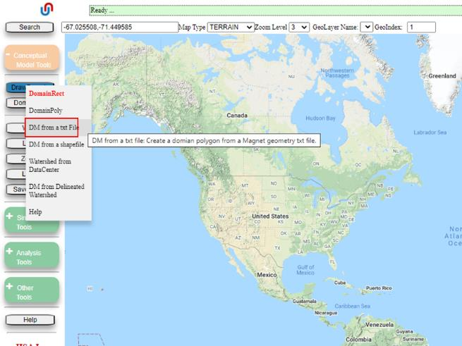
Domain.txt).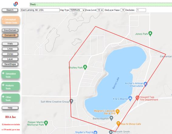
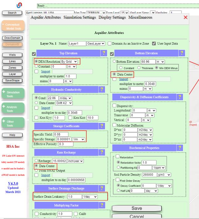
The aquifer parameters to assign at the domain level:
- Specific Yield: 0.08
- Conductivity: deferred to the DM zone (see step 2) — domain value is ignored
- Specific Storage: 1×10⁻⁶ 1/ft
- Top Elevation: DEM (default)
- Bottom Elevation: Data Center — Michigan aquifer thickness layer
- Surface Drainage Discharge: 1/day (default)
- Recharge: Data Center — Michigan spatial data layer
2. Import a T-PROGS 3D geology model as the conductivity field
The aquifer conductivity field comes from a pre-computed Transition Probability (TP) geostatistical model built from Michigan Wellogic borehole data. To apply it to the aquifer:
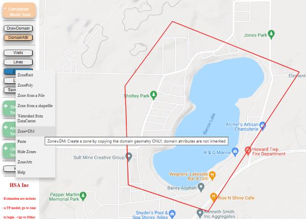
Create a zone with the same geometry as the domain using Conceptual Models Tools → Zones → Zone=DM — a "domain-matching" zone that inherits the domain geometry but can carry zone-specific attributes.
Inside the DM zone's Flow Properties, check Conductivity and select Borehole Simulation as the sub-option. Click the … options button to open Borehole Simulation Options. Check Import and browse to BarronLakeTP.tp (the T-PROGS result file). Assign typical x-direction conductivity values for the 4 material types identified by the geology model:
- Material 1: 53 ft/day (coarse sand/gravel)
- Material 2: 5 ft/day (fine sand)
- Material 3: 0.01 ft/day (silt/clay)
- Material 4: 0.001 ft/day (very fine clay/till)
Use defaults for Kxx/Kyy, Kxx/Kzz (horizontal isotropy, 10:1 vertical anisotropy).
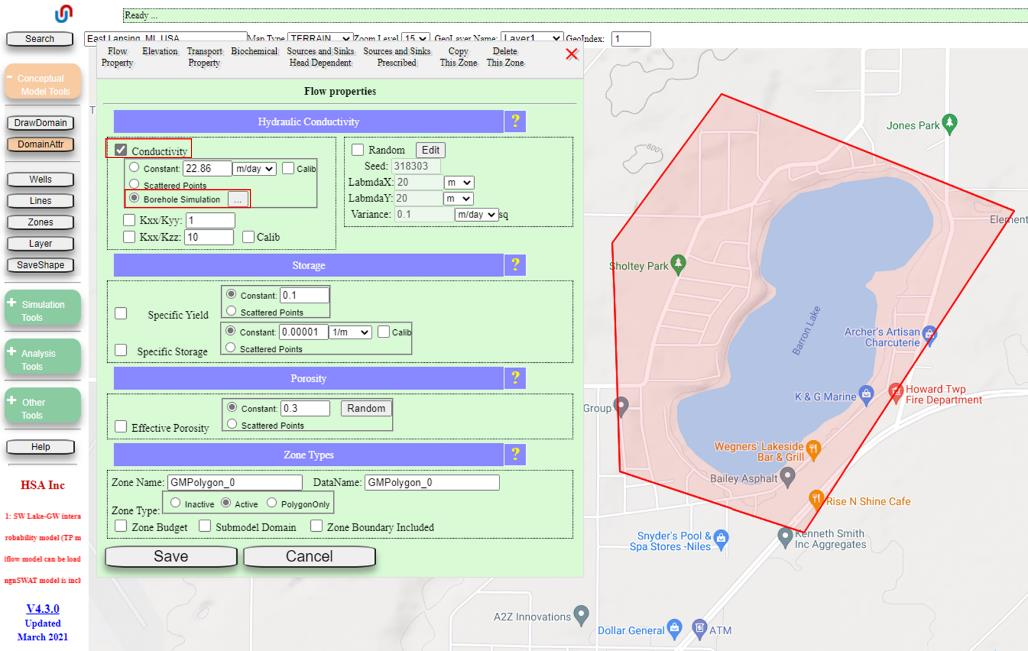
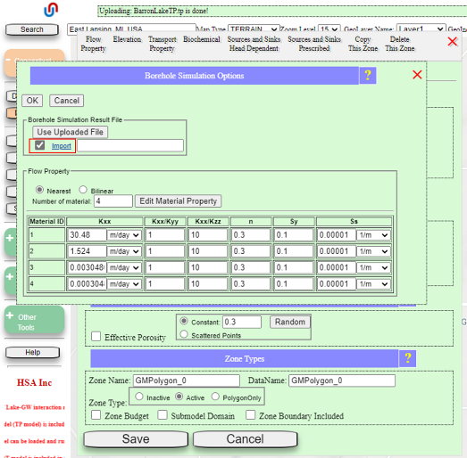
BarronLakeTP.tp loaded and material-specific K values assigned.3. Configure overland / watershed modeling
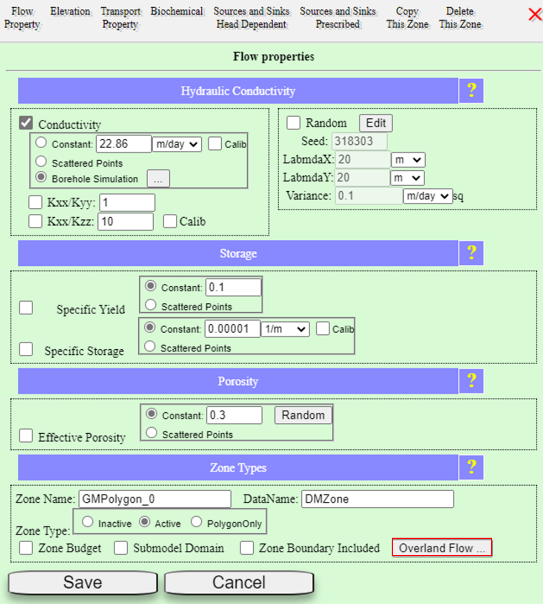
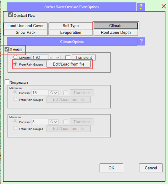
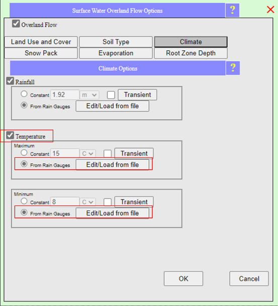
Still inside the DM zone's Flow Properties, click the Overland Flow… button towards the bottom-right. This opens the Surface Water Overland Flow Options menu. Check Overland Flow to direct IGW-NET to simulate land-surface hydrologic processes — runoff, recharge, evapotranspiration, snowpack dynamics.
- Land Use and Cover: raster from Data Center
- Rainfall: From Rain Gauges → From Data Center
- Temperature (min and max): from Data Center
- Soil Type: raster from Data Center; open Lookup Table and change all
CtaOvalues to −1.0 (this tells IGW-NET to pull initial soil moisture from a provided file rather than computing from type) - Root Zone Depth: raster from Data Center
- EVT: Priestley-Taylor Equation with default adjustment factors
- Snowpack: enabled with default parameters
4. Load the lake polygon
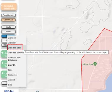
Load BarronLake.txt as a zone via the text-file import. Two prompts require attention: tolerance (for polygon smoothing) should be 0 (no smoothing applied); "delete all existing attribute zones" should be Cancel (keep the DM zone intact).
5. Parameterize the lake — two-way coupling with bathymetry and stage
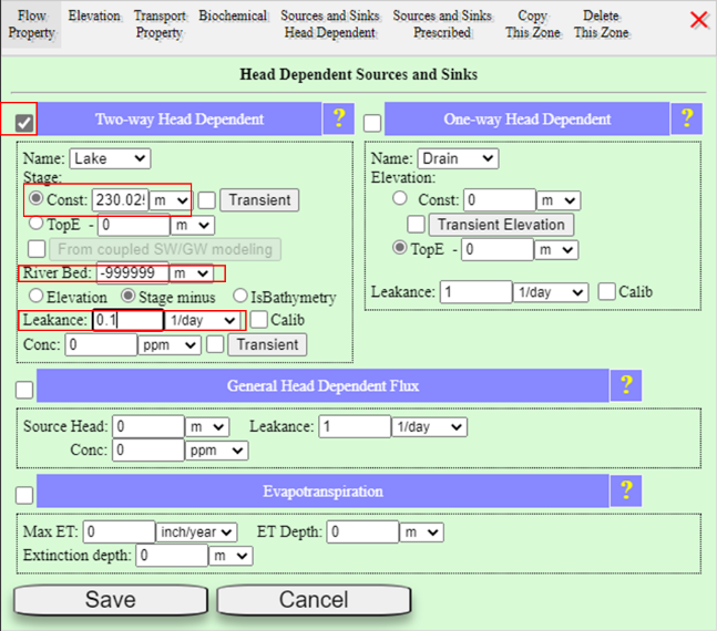
In the lake zone's Zone Attributes, navigate to the Source and Sinks Head Dependent tab and check Two-way Head Dependent. Configure:
- Initial lake level (Stage, Const): 230.0259392 m (from observations at simulation start)
- Leakance: 0.1 1/day
- River Bed:
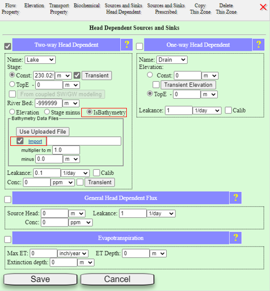
-999999(sentinel indicating a bathymetry file will be used; DEM is the reference) - IsBathymetry option: selected; Import
WaterDepth.txt - Stage: check
From coupled SW/GW modeling— this tells IGW-NET that stage is computed as part of the coupled process, not prescribed
Click the From coupled… button to open the Surface Water Source and Sink interface. Configure transient inputs:
- Under SW Prescribed Source/Sink, select
Transientand click…. LoadQsw.csv— the augmentation pumping into the lake. - Check SW Stage Measurement and click
…. LoadLakeLevel2013.csv— observed lake levels for validation.
6. Activate the Watershed Solver
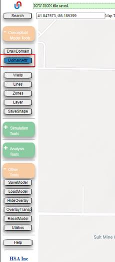
Open DomainAttr and navigate to Simulation Settings. Click the Watershed Solver button.
- Number of SW sub-time steps: 1 (one surface-water time step per groundwater time step)
- Import Initial Soil Storage: check Import; load
Cta0000.Tfirst, thenCta0000.V - SW Infiltration as GW Recharge: checked (couples SW infiltration directly into GW recharge)
- Overland flow solver: non-process-based (default)
7. Add the lake augmentation well
The augmentation well extracts water from the deep aquifer and delivers it to the lake — a common management strategy for small recreational lakes with marginal water balance. Draw a well anywhere using DrawWell, then correct coordinates in the Well Input Options menu:
- Latitude: 41.8479458145246
- Longitude: −86.1756223309731
- Transient pumping rate: check Transient, load
Qpumping.csv(the time-varying pumping rate)
8. Transient boundary conditions from a shapefile
Time-varying boundary conditions around the lake perimeter are based on regional flow patterns and water-level records at 11 private wells. They're modeled as transient "rivers" with very high leakance (mimicking prescribed-head BCs) but conceptualized as two-way head-dependent source/sink zones.
Import the shapefile
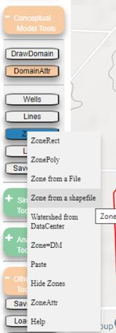
Conceptual Model Tools → Zones → Zone from a shapefile opens the Shapefile Import Options interface. Upload StagePolygons.shp, .dbf, .prj (all three required). Filter by MUNICIPLTY and select all entries. Click Next.
Under Select Attributes Options:
- Choose Used as Zone (more sub-options appear)
- Choose Shape-specified and select
MUNICIPLTYfrom the dropdown — each zone is named by its MUNICIPLTY entry - Check Two-way flux; group name
River(for mass balance differentiation) - Constant water depth: 1 m
- Constant Leakance: 5000 1/day (very high → mimics prescribed head)
- Click Add to MAGNET4WATER Model
Add time-varying stage to each zone
For each imported zone:
- Click
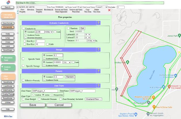
Other Tools → Utilities → Geometry unlock, then click inside the zone. A prompt confirms which zone was selected (by MUNICIPLTY name). - In Source and Sinks Head Dependent, check Two-way Head Dependent
- Choose Const, check Transient, click
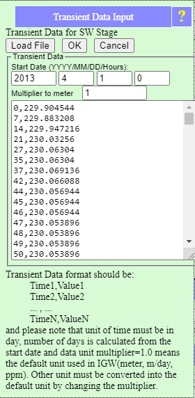
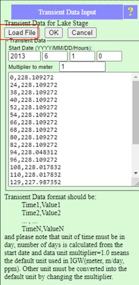
…to open Transient Data Input - Click Load File and browse to the appropriate stage CSV —
StageMyer.csv,StageKelly.csv, etc. - Copy the initial water level (first row), paste into the Const field — this sets the initial value for the transient simulation
- Click Save
9. Grid, layers, and transient flow settings
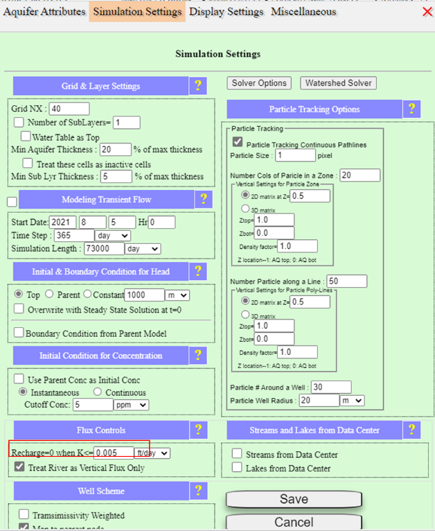
- Grid NX = 80 (80 cells in west-east direction)
- Number of SubLayers = 5 (checked)
- Modeling Transient Flow: checked
- Start date: 6/25/2013
- Time step: 1 day
- Simulation Length: 135 days
- Overwrite with Steady State Solution at t=0: checked (IGW-NET first solves steady state, then uses that as initial condition)
- Recharge threshold: Recharge = 0 when K ≤ 0.005 ft/day
10. Run and analyze the coupled simulation
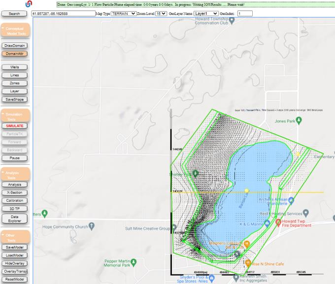
Simulation Tools → SIMULATE. Accept the suggested projection. The status bar reports progress; after the first time step (1 day) is solved, head contours and velocity vectors appear over the domain.
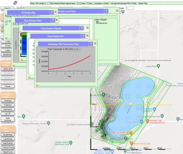
Analysis Tools → Analysis → Display Charts opens the full chart suite. Configurations of note:
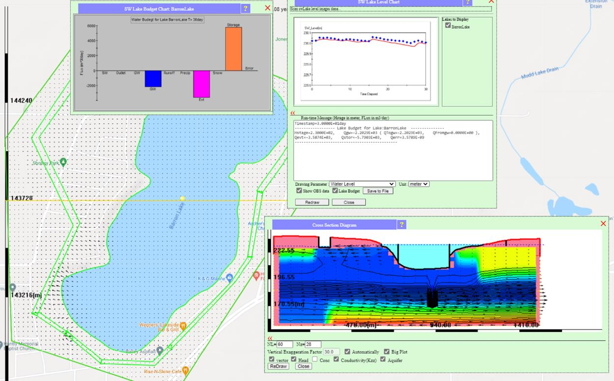
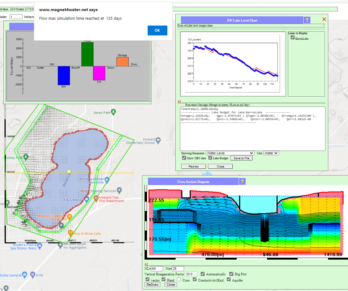
- In the Cross Section Diagram, enable Conductivity (Kzz) and Big Plot. Colors show vertical conductivity (red = high; blue = low), revealing the T-PROGS heterogeneity structure.
- In the SW Lake Chart, enable Show Obs Data and Lake Budget, then Redraw. This overlays the observed lake levels (from
LakeLevel2013.csv) on the simulated stage, and opens the Lake Budget Chart showing inflows and outflows.
Technical notes and advanced features exercised
This model exercises several advanced platform features that are each touched by individual quick tutorials but rarely combined. The coupling patterns are worth noting:
- T-PROGS ↔ groundwater flow: The 3D geologic model drives conductivity assignment. Material-specific K values are the user-supplied interpretation of the TP simulation.
- Watershed solver ↔ groundwater recharge: The
SW Infiltration as GW Rechargeflag converts watershed-scale infiltration into GW recharge directly, without user-supplied recharge rates. - Lake ↔ watershed ↔ groundwater: The lake receives runoff from the watershed solver, exchanges flow with groundwater through bathymetry-based leakance, and receives augmentation pumping as a direct SW input. All three are active simultaneously.
- Shapefile BCs ↔ private-well observations: The transient stage data at BC zones is inferred from private monitoring wells — the model's boundary conditions are data, not idealization.
Source Provenance
- Original document
- Barron Lake Integrated Model tutorial v1 (PDF)
- Site location
- Barron Lake, Niles, Michigan — approximately 41.85°N, 86.18°W
- Monitoring period
- Lake levels: 2006-2013 | Groundwater monitoring: 11 private wells, 2013–
- Simulation period
- 135 days starting 6/25/2013
- Geology source
- Michigan Wellogic borehole database; T-PROGS geostatistical realization (BarronLakeTP.tp)
- Platform
- IGW-NET / MAGNET4WATER with Watershed / Overland Flow Solver active
- Last reviewed
- 2026-04-20