The quick read — 90 seconds
- Nested modeling = finer ijk where xyz demands it. A parent regional model captures the big picture at moderate resolution; one or more child submodels resolve local features at finer resolution. The child uses the parent's computed heads as boundary conditions, so regional flow context flows automatically into the local simulation. See Ch. 1 §1.5.1 for the foundational framing.
- Two ways to create a submodel — the zone-based approach is preferred. Zone-based: draw a ZoneRect (or ZonePoly) in the parent, flag it in Zone Attributes as Submodel Domain (a bounding-polygon-only flag; the zone cannot also set physical attributes). Domain-based: use DrawDomain to draw a new smaller domain — but this erases the previous domain (IGW-NET holds only one domain at a time); the parent's boundary heads are captured into an internal exchange field before erasure, which is what gives the new domain its BCs. Both approaches require the Boundary Condition from Parent Model flag in Simulation Settings. The zone-based approach lets you keep multiple submodel candidates coexisting in the same parent and switch between them freely; the domain-based approach discards the parent from the session.
- The 10-cell sizing rule. The area of critical interest should sit at least 10 submodel-cells inside the boundary in every direction, because inherited-BC artifacts propagate inward a few cells before regional flow takes over. This rule drives how big each submodel has to be.
- Watch out — silent failure from multiple active submodel zones. Only one submodel zone can be active at a time. If you draw a new zone without first unchecking the previous one's Submodel Domain flag, the new zone has no effect — the platform keeps using the old one, and you get the wrong results without any error. Treat the Submodel Domain flag like a radio button: uncheck the previous zone before checking the new one. See §13.7.5.
- Why nesting beats just refining NX. Compute cost scales with the square (or cube in 3D) of resolution. Uniformly doubling NX quadruples total cells — most of which are in areas you don't need fine detail. A 5 km × 5 km submodel at NX = 80 inside a 100 km × 100 km parent at NX = 40 is roughly 1% of the cost of uniformly refining the parent to match.
- BCs inherit; interior features don't automatically. The submodel gets its lateral boundary heads from the parent's flow solution. Optionally, starting heads too. But the interior conceptual features (wells, zones, polylines, layer definitions) are yours to refine in the submodel — add detail the parent didn't have, represent features at finer resolution.
- Hierarchy is fundamental, not just efficient. Many small models solve more robustly than one big one (numerical), humans assimilate hierarchically (cognitive), managers make decisions at different scales (management), and hierarchical data fits internet delivery (infrastructure) — all four reasons independently point to hierarchy as the right framework. The 10-cell rule plus large scale disparity often forces multiple levels on top of that. Regional → watershed → site → plume-area nesting is standard for serious site investigations. Each level is light; the zone-based approach keeps all levels navigable. See §13.5.1 for the full argument.
- Place the submodel boundary carefully. Keep it away from the parent's active features (pumping wells, complex surface water) and away from the parent's own outer edge where parent heads are least reliable. A submodel abutting the parent boundary inherits the parent's no-flow-boundary artifacts.
- MODFLOW-6 unstructured refined grid is a different refinement mechanism, and the choice between the two is about scale disparity. Use nested submodels when regional context and area of interest differ by ~100× (regional 100 km with local 1 km). Use unstructured refined grid when your domain and features are the same scale but you need better numerical representation around specific features within a single, same-scale domain (§13.6).
13.1 Why Nest — The xyz/ijk Argument
Nested modeling is not just a convenience — it is the direct consequence of the conceptual-versus-numerical distinction introduced in Chapter 1 §1.5.1. This section lays out the reasoning explicitly, because understanding why you nest makes the when and how clearer.
13.1.1 The core problem — single-grid inadequacy
Real aquifer systems span scales: a regional flow pattern driven by climate, topography, and regional geology; a local flow pattern affected by specific wells, streams, and small-scale heterogeneity. A single numerical grid (ijk) has one resolution — every cell in the domain is the same size. If you set that resolution coarse enough to keep the regional model computationally tractable, the local features are under-resolved. If you set it fine enough to resolve local features, the regional computation is wasteful (most of the fine cells are in areas where coarse cells would suffice).
This is a fundamental tension between ijk and xyz. The conceptual reality (xyz) naturally has multi-scale structure. A single-resolution numerical representation (ijk) cannot honor both regional and local scales simultaneously. Nested modeling resolves the tension by using multiple ijk representations — a coarse one for regional context, a fine one for local detail — linked through boundary-condition inheritance.
13.1.2 The compute-cost argument
Grid cost scales roughly with the square (2D) or cube (3D) of resolution. Doubling NX from 40 to 80 quadruples the 2D cell count; doubling sublayers from 1 to 2 and NX from 40 to 80 octuples the 3D cell count. Most serious simulations scale superlinearly with cell count because the solver iterations multiply. The practical effect: uniformly refining a large domain to get local detail is expensive, often prohibitively so.
| Approach | Region cells (NX = 40) | Local cells (NX = 80) | Total cells | Relative cost |
|---|---|---|---|---|
| Uniform parent at NX = 40 | 40 × 40 = 1,600 | (local inside parent) | 1,600 | 1× |
| Uniform parent at NX = 80 | — | — | 80 × 80 = 6,400 | 4× |
| Parent NX = 40 + submodel (5% of domain) at NX = 80 | 1,600 | 80 × 80 × 0.05 ≈ 320 | 1,920 (two runs) | ~1.2× |
| Parent NX = 40 + submodel at NX = 160 | 1,600 | 160 × 160 × 0.05 ≈ 1,280 | 2,880 (two runs) | ~1.8× |
The nested approach delivers arbitrary local resolution for a cost that's only a small multiple of the parent-alone cost. This is the efficiency that makes very-fine local simulations practical in IGW-NET even on a web-based platform.
13.1.3 When a submodel is worth creating
You want a submodel when:
- A local feature needs finer resolution than the parent's grid provides. A pumping well, a specific source zone, a detailed stream network, a plume area. The parent resolves the regional flow well enough; you need to zoom in on the local structure.
- You're doing site-specific transport in a regional flow context. Standard for any contamination investigation with regional implications — the local source and plume need fine-grid transport while the regional groundwater divides and streams remain in the parent.
- You want WHPAs or GDE recharge areas with defensible resolution. A WHPA delineation demands sharper cell resolution near the well than a regional parent can economically provide (Ch. 11 §11.5.2).
- Your calibration is local, but your physics is regional. You have monitoring data at a site; you need flow calibrated locally. A submodel gets the regional drivers right automatically (via BCs) while you tune local K and layer detail.
- You need to compare scenarios at a site. Running alternative local configurations is cheap because the parent solution can be reused; each submodel variant is a short simulation against the same parent flow field.
Use a submodel when the xyz-conceptual reality has important local structure that the parent's ijk resolution blurs. The submodel's finer ijk honors the xyz more faithfully in the area you care about, while the parent keeps the regional context correct. This is the platform-specific expression of the "where does ijk need to be faithful to xyz?" question framed in Ch. 1 §1.5.1 and Ch. 7 §7.3.
13.2 The Submodel Workflow — Two Approaches
IGW-NET offers two distinct ways to create a submodel: the zone-based approach (ZoneRect + Submodel Domain checkbox) and the domain-based approach (DrawDomain inside the parent area). Both link to the parent through the Boundary Condition from Parent Model flag, and both produce the same submodel simulation. They differ in workflow convenience and in what they let you do afterward. This section walks through each approach and explains when to use which.
13.2.1 Prerequisite — a converged parent model
Before creating any submodel, you need a converged parent — your regional model with domain drawn, attributes configured, features defined, and a successful SIMULATE. Check the water balance (Ch. 8), confirm head contours look physically reasonable, and confirm there are no error messages. The submodel's BCs come from the parent's computed heads, so if the parent is poorly calibrated or badly gridded where the submodel will be, those errors propagate into the child. Spend the time on parent calibration first.
Before choosing an approach, know what size your submodel needs to be. IGW-NET's rule of thumb is that the area of critical interest should be at least 10 cells inside the submodel's boundary, in every direction. BC artifacts from the inherited fixed-head boundary propagate inward a few cells before regional flow patterns take over; 10 cells gives a safe buffer for most situations. If your submodel is NX = 40 with a 4 km × 4 km domain (100 m cells), your area of interest should sit in the inner ~2 km × 2 km. If your target zone is larger than that, enlarge the submodel.
This rule shapes how you size every submodel — and, when the scale disparity between regional parent and local area is extreme (100× or more), it is why you often need a hierarchy of submodels rather than a single level (see §13.5).
13.2.2 Approach A — The zone-based workflow (recommended)
The zone-based approach is IGW-NET's preferred workflow for submodels. You draw a zone in the parent model, flag it as a Submodel Domain, and the platform treats that zone as the active simulation domain when BC-from-parent is enabled. Here is the full procedure:
Draw a zone with ZoneRect or ZonePoly
Click Conceptual Model Tools → Zones → ZoneRect (or ZonePoly if you want an irregular submodel boundary). Click corners on the map to define the zone's geometry. Apply the 10-cell buffer rule above when sizing.
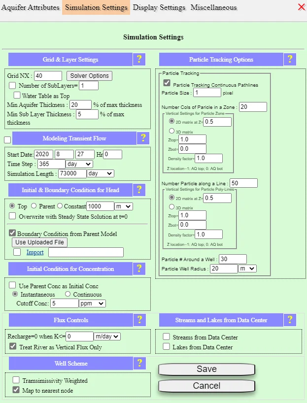
SaveShape and check Submodel Domain in Zone Attributes
Click SaveShape. The Zone Attributes dialog opens. In the default "Flow Property" tab, find the Zone Types subsection and check the Submodel Domain box. Click Save.
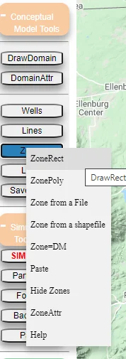
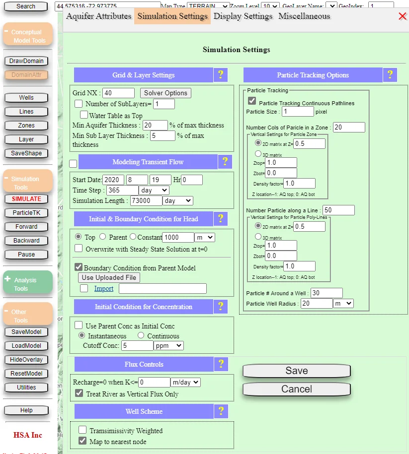
Enable BC from Parent Model in Simulation Settings
Click Conceptual Model → Domain Attributes → Simulation Settings, and check Boundary Condition from Parent Model. Click Save.
SIMULATE
Click SIMULATE. The platform steps through three confirmation prompts (accept each one); the submodel simulation begins at its finer resolution with parent heads as BCs.
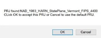
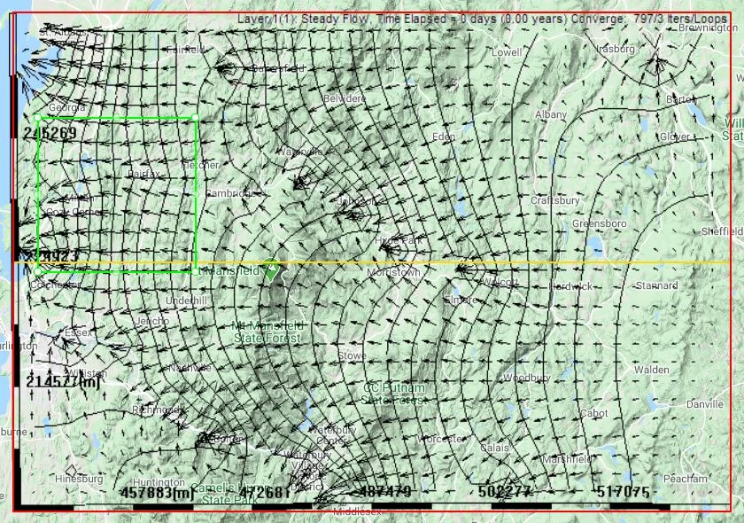
You can have multiple rectangles or polygons all checked as Submodel Domain living in the same parent at once. Each zone persists — its geometry and location are saved in the parent model — but only one is "active" at any simulation. When you click SIMULATE, IGW-NET asks which submodel zone to use. This lets you define several candidate submodel regions (a plume area, a wellfield, a surface-water impact zone, a hypothetical future-development area) and switch between them without redrawing. Switching is free: you change which submodel is active, click SIMULATE, and the platform runs whichever zone you picked. Your domain polygon (the parent) is always preserved, so you can flip back to regional view any time by clearing the Submodel Domain flags or unchecking BC-from-parent.
Important caveat — the "silent failure" trap: only one submodel zone is active at a simulation. If you draw a new submodel zone without first unchecking the previous one's Submodel Domain flag, the new zone has no effect — the simulation continues to use whichever zone was previously active, and you see the wrong results without any error. The defensive habit: treat the Submodel Domain flag like a radio button. Always uncheck the zone you're moving away from before checking the new one. See §13.7.5 for more on this pitfall.
13.2.3 Approach B — The domain-based workflow
The second approach uses DrawDomain to create a new, smaller domain inside the area the parent covered, then references the parent for BCs. The workflow:
- With the parent model converged, click Conceptual Model Tools → DrawDomain and draw a new domain polygon in the area of critical interest (e.g., the remediation site). Apply the 10-cell rule when sizing. When you commit the new domain, the previous parent domain is erased — IGW-NET only ever holds one active domain at a time — but the parent's boundary-head values at the new domain's perimeter are captured into an internal exchange field before the erasure.
- Attributes for the new domain are populated from the Global Base Model (not from the parent, which is gone).
- In Simulation Settings, check Boundary Condition from Parent Model. This tells IGW-NET to read BCs from the saved exchange field rather than defaulting to no-flow.
- SIMULATE. The new, smaller domain runs with fixed-head BCs sourced from the exchange field.
This is the crucial operational difference between the two approaches. IGW-NET's conceptual model holds exactly one domain polygon at any time. When you DrawDomain, the previous domain is gone — you cannot simply re-simulate the parent afterward, because the parent's domain no longer exists in the session. What does persist is the exchange field — the snapshot of parent-computed boundary heads taken at the moment of erasure. That snapshot is what enables the new, smaller domain to run with realistic BCs without the parent model still being there.
Consequences worth being deliberate about: (a) to return to regional view, you must reload the parent's saved model file; (b) to move to a different local area, you must redraw — and when you do, the current submodel's exchange-field BCs are replaced with a new snapshot sourced from... wherever the current head field happens to be, which may not be what you want; (c) regular saving of the parent model before using DrawDomain is essential with this approach.
13.2.4 Choosing between the two approaches
| Approach | Best for | Watch out for |
|---|---|---|
| Zone-based (Approach A) | Most work. Pre-defining multiple candidate submodel regions. Switching between regional and local views freely. Iterative investigations where the area of interest may shift. Hierarchical nesting (§13.5) where each level needs its own preserved submodel zone. | The zone-as-Submodel-Domain is a bounding polygon only — you can't also use it to set physical attributes or stresses. If you need a feature zone and a submodel boundary in the same area, use two separate zones. Only one submodel zone can be active at a time — see §13.7 for the multiple-zone pitfall. |
| Domain-based (Approach B) | One-off quick investigations. When you know you only need to look at one specific submodel and have no reason to preserve the regional parent in the session. Cases where you're rebuilding the conceptual model substantially and prefer a fresh domain populated from the Global Base Model. | DrawDomain erases the previous domain — the parent is gone from the session once you draw the new one. BCs persist via the exchange field, but the parent's geometry, features, and attributes do not. Always save the parent before DrawDomain. |
For most practical work — and especially for any investigation involving hierarchical nesting or comparison between candidate submodel locations — the zone-based approach is strongly preferred. The domain-based approach has its place but erases what came before.
13.2.5 The visual check — reading the submodel solution
The single quickest check that your submodel is using parent BCs correctly: look at how head contours intersect the submodel's outer boundary. Contours orthogonal (perpendicular) to the boundary indicate no-flow BCs — parent inheritance is NOT working. Contours that cross the boundary at angles indicate directional flow through the boundary — parent inheritance IS working. If you see the orthogonal-contour pattern, recheck that the Boundary Condition from Parent Model flag is on and the Submodel Domain zone (if using Approach A) is checked.
13.2.6 Switching back to the parent
With the zone-based approach: uncheck Boundary Condition from Parent Model in Simulation Settings (or uncheck Submodel Domain on the zone), then SIMULATE. The platform returns to parent mode and uses the full parent domain. You can toggle freely — each has its own grid and its own simulation.
With the domain-based approach: you need to load the parent's saved model file, since the current domain has been replaced.
13.3 What Inherits, What Doesn't
Understanding exactly what the submodel gets from the parent — and what you still need to specify yourself — is essential to using submodels correctly. The rule of thumb: boundary conditions inherit automatically; interior representation is yours to refine.
13.3.1 What inherits automatically
| What inherits | Mechanism |
|---|---|
| Lateral boundary heads | Parent's computed head field, interpolated to the submodel's perimeter cells, becomes fixed-head BCs. Required by the submodel workflow. |
| Bottom boundary (for unconfined models) | Inherits the parent's layer configuration by default; default no-flow if nothing specified differently. |
| Starting head (optional) | Separate flag (Head from Parent Model) — when enabled, the submodel's initial head distribution is interpolated from the parent's final solution, giving faster convergence for transient runs and for steady-state runs with significant gradients. |
| Regional data context | Data Center rasters (Ch. 4), Global Base Model attributes, DEM, and other global data sources are the same in the submodel as in the parent — the submodel is still a piece of the same xyz reality. |
13.3.2 What does NOT inherit automatically
The submodel is an opportunity to refine the representation, not just copy it. So interior features are yours to define — potentially differently from how they appeared in the parent:
| What doesn't inherit | What to do |
|---|---|
| Interior zones | Zones drawn in the parent appear visually in the submodel but are not actively represented unless you explicitly keep them. You can refine zone boundaries, add detail zones the parent didn't have, adjust attributes to local data. |
| Interior wells | Wells inside the submodel domain should be re-examined — sometimes you add wells to the submodel that weren't in the parent (because they were below the parent's resolution), or you refine pumping rates for the local study. |
| Polylines (streams, drains) | Regional streams stay; detailed local streams can be added at submodel resolution. A stream that the parent represented as a simple polyline may become a detailed, segmented stream in the submodel. |
| Layer count and sublayer count | The submodel can have different vertical resolution than the parent. A parent at 1 sublayer can host a submodel at 10 sublayers for 3D transport analysis (Ch. 12 §12.4.7). |
| Grid NX | The submodel has its own NX — typically 2× to 4× the parent's, sometimes more. This is the point of nesting. |
| Aquifer attributes | The submodel can have different dispersivity, sorption, decay, and other transport parameters if your local study calls for values that differ from parent-scale defaults. |
| Transport sources | Source zones, injection-well concentrations, and other transport sources must be defined in submodel mode to be active. Parent-scale transport setups don't automatically carry into the submodel. |
| Particles | Particle placement is specific to whichever model is active. Particles you placed in the parent for a regional analysis are not the particles you use in the submodel for a local analysis. |
A submodel is a new simulation with new freedom — to add detail, to refine boundaries, to use different attributes where local data warrant. Treating it as merely "parent displayed at higher resolution" misses the point. The whole reason to nest is to represent the xyz reality more faithfully in the area of interest, which typically means adding to what the parent had, not just copying it.
13.3.3 Keeping parent and submodel in sync
Changes to the parent (e.g., a new well added regionally, a changed recharge rate, a re-calibrated K field) can affect the submodel's BCs. When you change the parent, re-SIMULATE the parent to update its flow solution, then re-SIMULATE the submodel so it picks up the new BC values. The platform does not automatically propagate parent changes into submodel results — the submodel's BCs are from the parent's last-solved state.
This usually isn't a problem during active model development (you're iterating on one level at a time), but it's worth knowing. A stale submodel solution that shows "wrong" heads at its boundaries is often just a submodel that hasn't been re-simulated since the parent was updated.
13.4 Placing the Submodel Boundary
Where you draw the submodel's outer rectangle matters. The parent's computed heads along that rectangle become the submodel's boundary conditions — so if the parent's heads are unreliable there, the submodel inherits the unreliability.
13.4.1 Rules of thumb
| Rule | Why |
|---|---|
| Leave at least 10 submodel cells between the boundary and the area of critical interest | Inherited BCs introduce small artifacts that propagate inward a few cells before regional flow patterns take over. Ten cells of buffer gives the solution space to recover. If your submodel is NX = 40 with 100 m cells, the area of interest should sit at least 1 km in from every edge. This is the dominant sizing rule — it often determines how big the submodel needs to be, and it is why severe scale disparity requires a hierarchy of submodels rather than a single level (§13.5). |
| Keep the submodel boundary away from the parent's own outer edges | The parent's edges are themselves BC-constrained; heads there are artifacts of the parent's BCs, not of regional flow. A submodel abutting the parent edge inherits these artifacts. |
| Keep the submodel boundary away from pumping wells in the parent | Near wells, the parent's coarse grid can't resolve the cone of depression accurately. Submodel BCs here will be smeared approximations of the real head field. |
| Align the submodel boundary with low-gradient areas when possible | Errors in parent heads translate directly into BC errors. In low-gradient areas, parent heads are better-determined and more robust to small calibration errors. |
| Avoid placing the boundary across major surface-water features | A stream running through the submodel's boundary creates a sharp head discontinuity the parent may handle differently than the submodel does. Put the boundary upstream or downstream of the feature. |
13.4.2 Exception — when an edge coincides with a natural boundary
A useful exception to the "away from edges" rule: if a natural hydrologic boundary (a major river, a lake, a groundwater divide) coincides with a parent edge, a submodel boundary there is fine — even helpful. The parent's head at the river is controlled by the river itself (through surface-water coupling), so parent-heads there are physically meaningful and defensible. The submodel inherits a physically-grounded BC rather than an artifact. Example: a parent whose western edge is a major lake can host a submodel whose western edge is the same lake without penalty.
13.4.3 Iterating to find a good boundary location
Draw a trial submodel
Place the submodel boundary where it seems reasonable. Simulate.
Check the area of interest
Does the solution in the area you care about look physically sensible? Are contours smooth? Do they agree with parent contours at overlap?
If results look suspicious at the submodel boundary, move the boundary further out
If contours bend sharply at the boundary, if mass balance shows unexpected fluxes at the boundary, or if head values at the boundary look inconsistent with parent values there, enlarge the submodel so the artifacts move out of the area of interest.
Re-simulate; check again
Larger submodel is slower but more reliable. Balance cost versus BC-proximity sensitivity.
13.5 Hierarchies — Submodels Inside Submodels
A submodel can itself host a submodel. This nesting can continue to arbitrary depth in principle, though three to four levels is the practical maximum in most applications. Hierarchical nesting is how IGW-NET handles genuine multi-scale problems where the xyz reality has structure spanning many orders of magnitude. But the case for hierarchy is stronger than "it handles multi-scale problems" — hierarchy is the right organizing principle for modeling, assimilation, visualization, and data transmission simultaneously. This section starts with the deeper argument, then works through the operational specifics.
13.5.1 Why hierarchical modeling is fundamental, not just efficient
Nested modeling is often framed as a numerical trick — a way to avoid building an enormous single grid. That framing undersells it. Hierarchical organization is fundamentally the right way to represent and work with multi-scale information, for reasons that go far beyond compute cost. Four arguments, each independent, each pointing the same direction:
Numerical — many small models solve more robustly than one big one
A single monolithic model covering multiple scales at uniform fine resolution is numerically harder than the sum of its nested equivalents. Large grids produce large, ill-conditioned linear systems; convergence slows non-linearly with problem size; coupled failure modes (one region's problem cascading into the whole solution) become more common. A three-level hierarchy of small, well-posed problems is more robust at every level: each individual solve converges faster, each is independently diagnosable, each can be re-simulated in seconds rather than minutes. If the plume-area sub-submodel has a convergence issue, it's isolated — the regional and watershed solutions stay clean. In a monolithic model, the same issue could contaminate the whole field, and diagnosis requires picking through a million-cell solution to find where things went wrong.
Cognitive — humans assimilate hierarchically, not pixel-by-pixel
Even if the machine can solve a monolithic model perfectly, a human user cannot assimilate the result as a flat field of values. Comprehension is hierarchical: first the overall pattern (regional flow direction, major discharge areas), then the intermediate structure (watershed-scale features, local flow convergence), then the details (plume shape, individual well capture). Looking at a million head values at uniform resolution overwhelms the eye and the mind. A hierarchy of views — regional at coarse resolution, site at moderate resolution, plume area at fine resolution — matches how humans build understanding. Each level presents about as much information as comprehension can absorb at that scale; the finer levels carry the detail that would have been noise at coarser levels and clutter at monolithic resolution.
Management — decisions are made hierarchically
Different stakeholders in a real groundwater study need different views. A regulator wants to know whether the aquifer system is protected — regional-scale answer. A site manager wants to know whether this site's remediation is on track — site-scale answer. A plume-response engineer wants to know whether the extraction well is capturing the plume — plume-scale answer. These are the same physical system, examined at different levels of detail. A single monolithic model tries to answer all three at once and ends up being unwieldy for each. Hierarchical models match the decision structure: the right level of detail reaches the right decision-maker without requiring everyone to work with full-resolution data. This is how organizations have always structured technical information — executive summary, technical report, detailed appendix — and modeling deliverables work the same way.
Infrastructure — hierarchy matches how data transmits across the internet
Modern groundwater work is browser-based, collaborative, and distributed. Transmitting a million-cell uniform model over the internet, to a browser, for a user to interact with, is impractical — the bandwidth cost is real, the render cost is real, and the interaction latency kills productivity. Hierarchical models transmit only what the current view needs: a coarse regional field when looking at regional scale, finer fields when you zoom in, full detail only for the sub-area currently in focus. This matches how web-based mapping has always worked (Google Maps doesn't send you all the world's tiles at every zoom level) and how cloud-native scientific computing increasingly works. IGW-NET's streaming-visualization architecture assumes hierarchy — it is how the platform achieves the responsive, interactive feel it does. A non-hierarchical representation would not fit the delivery medium.
These four arguments — numerical, cognitive, management, infrastructure — are independent and unanimous. Even if any one of them didn't apply, the others would still point to hierarchy. When all four point the same way, the conclusion is not that hierarchy is a useful optimization; it is that hierarchy is the right framework for modeling, assimilation, visualization, and data transmission. Monolithic single-scale models are the exception, not the default. The modeling platform, the cognitive load on users, the management of decisions, and the network that carries the data all want hierarchy.
IGW-NET's nested-submodel workflow is the expression of this principle in the platform. When you build a hierarchy of submodels, you are not just optimizing compute — you are organizing the modeling work the way the modeling work wants to be organized.
A common instinct among students, novices, and even experienced practitioners coming from other platforms is that cranking NX higher produces a better model. Push NX to 200, 300, 500 — surely finer is better? This instinct is mostly wrong, and acting on it is one of the most common real mistakes in applied groundwater modeling. Going brute-force usually means long runtimes, degraded convergence, or outright solver failure (a failed high-resolution run gives you nothing — not even a coarse answer). Even when it succeeds, much of the fine-grid compute was spent in areas that didn't need detail.
The better practice is to stay well within convergence-friendly NX limits (typically 100–150 or less in IGW-NET) and use hierarchy to get local fine resolution where it's actually needed. Each level of a hierarchy stays well-posed numerically; together they span whatever scale range the problem has — often more scale range than a monolithic model could handle at any NX. The mental shift is from "raise NX to resolve detail" to "use hierarchy to place detail where it matters." See Ch. 7 §7.3.2 for the specific discussion of why raising NX aggressively hurts more than it helps.
13.5.2 Why the 10-cell rule often forces a hierarchy
Beyond the four fundamental arguments in §13.5.1, there is a specific technical reason the hierarchy is often required rather than just preferred: the 10-cell-buffer rule from §13.4 cannot be satisfied in a single submodel level when scale disparity is severe. Consider what happens with a 1000× scale disparity — a 100 km × 100 km regional parent and a 100 m × 100 m area of critical interest:
- If you try to jump directly from the regional parent to a submodel tight around the 100 m area, the submodel must be much larger than 100 m — the 10-cell rule says the area of interest needs ~10 submodel-cells of buffer on each side. At NX = 40 covering 1 km (100 m cells), that 10-cell buffer only gives you a few hundred meters of breathing room. That's still acceptable — but the submodel is now a 1 km × 1 km domain that is being reached directly from a 100 km × 100 km parent, a 100× jump in scale.
- That 100× scale jump is at the edge of what parent BCs can reliably support. Parent cells at NX = 40 over 100 km have 2.5 km cell size; BCs interpolated from 2.5 km cells to a 100 m submodel edge are being stretched across 25× resolution mismatch. Contour discontinuities, head interpolation errors, and BC artifacts can become noticeable.
- The solution is an intermediate level: put a 10 km × 10 km watershed submodel between the regional parent and the plume-area sub-submodel. Now the regional-to-watershed jump is 10× (manageable), and the watershed-to-plume jump is another 10× (also manageable). The 10-cell rule is satisfied at each level because each level only needs to buffer against the next-coarser level's cell size, not against the regional parent's.
In short: huge scale disparity forces a hierarchy, because a single submodel level cannot simultaneously satisfy the 10-cell buffer rule and avoid stretching parent BCs across too large a resolution mismatch. The hierarchical workflow is the natural answer — and the zone-based approach in §13.2.2 (multiple submodel zones coexisting) is the platform feature that makes multi-level hierarchies practical to build and navigate.
13.5.3 The typical three-level hierarchy
| Level | Typical scale | Resolution | What it captures |
|---|---|---|---|
| Regional parent | 50–200 km × 50–200 km | NX = 40, 1 sublayer | Regional flow divides, major aquifer boundaries, regional recharge patterns, dominant surface-water features |
| Site / watershed submodel | 5–20 km × 5–20 km | NX = 80, 3–5 sublayers | Watershed-scale flow, local streams, site-scale geology, pumping wells, regional-to-local transition |
| Plume-area sub-submodel | 0.5–2 km × 0.5–2 km | NX = 160, 10+ sublayers | Plume shape and concentration, near-field source behavior, DNAPL or dense-plume vertical structure, detailed remediation capture zones |
Each level inherits its BCs from the next-coarser parent. The plume-area sub-submodel sees detailed local features (source, pumping wells, monitoring network) at high resolution, while its BCs are shaped by the site-scale watershed model, which in turn was shaped by the regional parent. Regional information flows down through the hierarchy to the most-detailed level without being lost in grid coarsening.
13.5.4 Why this works — the light-weight advantage
Each level of the hierarchy is a single, light simulation. The plume-area sub-submodel at NX = 160 with a 1 km × 1 km domain has 160 × 160 = 25,600 cells — large but not excessive. The watershed submodel at NX = 80 with a 10 km × 10 km domain has 6,400 cells. The regional parent at NX = 40 with a 100 km × 100 km domain has 1,600 cells. Each individual simulation is fast; together they cover five orders of magnitude in spatial scale with local resolution a thousand times finer than the regional.
Compare to a single unified grid covering the same 100 km × 100 km at 62.5 m resolution (matching the plume-area's NX = 160 on a 1 km subdomain): you'd need 1600 × 1600 = 2.56 million cells. That's 160× as many cells as the entire three-level hierarchy combined. The hierarchical approach is a fundamental efficiency, not a marginal optimization.
The regional parent carries information about continental or basin-scale context — divides, major recharge, dominant surface-water features. The watershed submodel carries information about catchment-scale hydrogeology — local streams, geologic units, pumping wells. The plume-area sub-submodel carries information about specific local features — source geometry, plume structure, monitoring-well capture. A single-grid model at any uniform resolution loses information at one scale or another: at coarse resolution, local detail is smeared out; at fine resolution, the domain has to shrink to stay tractable, and regional context is lost. The hierarchy keeps all scales of information visible in the form they should be visible — each level presenting roughly the right amount of information for that level's purpose, without over-detail that obscures or under-detail that misleads. This is the cognitive and management argument from §13.5.1 operationalized.
13.5.5 Practical workflow for a hierarchy
Build and calibrate the regional parent first
The parent's quality determines everything downstream. Calibrate against regional head data; confirm water balance; confirm flow directions match regional observations. Do this at NX = 40 — refining later wastes time if the coarser model has fundamental issues.
Add and simulate the watershed submodel
Draw the watershed-scale rectangle as a Submodel Domain zone in the parent. Enable BC from Parent. At this level, consider whether vertical resolution is still adequate — most watershed-scale submodels benefit from 3–5 sublayers (with Water Table as Top enabled; see Ch. 7 §7.4.3) to capture the vertical flow components that become meaningful at finer horizontal resolution. SIMULATE. Calibrate at this level against local head data and (if available) stream baseflow data. Add detailed surface-water features the parent lacked.
Add and simulate the plume-area sub-submodel
Switch to submodel mode (watershed as active). Now in watershed-mode, draw a smaller rectangle inside the watershed. Make that a Submodel Domain zone. At this level, increase sublayers further — typically 5–10 for general site-scale work, 10+ if you have depth-specific monitoring data, DNAPL behavior, or other vertical structure to resolve. Keep Water Table as Top checked. Simulate with BC from (now-)Parent Model. This is your plume-area simulation, inheriting BCs from the watershed, which inherited from the regional.
Iterate when data come in
New observations at any level can require recalibration at that level and re-simulation of all levels below it. The platform makes this manageable because each individual simulation is fast.
Each level of the hierarchy adds horizontal resolution (finer NX) — but horizontal refinement alone is rarely enough. The reason you refined horizontally is usually because local detail matters, and local detail almost always has a vertical component too: partial-penetration wells capture specific depths, contaminant sources release at specific elevations, streams discharge to specific aquifer horizons, and plumes develop depth-structured concentration patterns. So each level of the hierarchy typically has both finer NX and more sublayers than its parent.
When adding sublayers at finer levels, always enable Water Table as Top (Ch. 7 §7.4.3). Without it, naive DEM-based subdivision produces chaotic sublayer thicknesses and dry cells that crash the solver. With it, the platform uses the water-table solution from the previous simulation as the top of the uppermost sublayer — every sublayer stays fully saturated, the linear system stays well-posed, and convergence is fast. One or two iterations of the water-table exchange field usually suffice to reach a stable 3D solution.
In principle the hierarchy can go deeper — sub-sub-sub-models — but beyond three levels the overhead of coordinating multiple nested BCs usually outweighs the benefit. Three levels is enough for the vast majority of real problems.
13.6 MODFLOW-6 Unstructured Refined Grid — The Alternative Approach
IGW-NET offers a second refinement mechanism besides nested submodels: unstructured refined grid, a MODFLOW-6 feature that refines cells locally within a single simulation rather than creating a separate child. This section covers when each approach fits.
13.6.1 What unstructured refined grid does
Standard structured grids have uniform cell size throughout the domain. Unstructured grids allow cell size to vary — cells near specific features (wells, polylines, or zones you flag for refinement) are finer, and cells far from those features are coarser. The entire grid is one simulation in the MODFLOW-6 DISV (Discretization by Vertices) engine; you don't switch between parent and child models.
In IGW-NET, you flag specific features for refinement by setting their "isRefined" property through the feature's attribute dialog. When MODFLOW-6 is the active solver, the platform builds an unstructured grid that refines locally around each flagged feature.
13.6.2 When to use refined grid versus nested submodels
The real decision rule is about scale disparity — how different are the scales you're trying to simultaneously resolve?
- Significant scale disparity (regional vs local, orders of magnitude different) — use nested submodels. A 100 km × 100 km regional context with a 1 km × 1 km area of interest is a 100× scale disparity; a 10 km × 10 km site with a 100 m × 100 m source zone is a 100× disparity. Each level of a nested hierarchy gets its own grid tuned to its own scale, and you can examine each scale independently.
- Same scale, larger domain, need better feature representation locally — use unstructured refined grid. When the domain is relatively large (say 10–20 km across) but you need finer numerical resolution around specific features — a few wells, a meandering stream reach, a specific zone boundary — DISV refines cells locally while keeping the rest of the domain at reasonable resolution. One simulation, one coherent grid, refinement where features live.
| Use unstructured refined grid when... | Use nested submodels when... |
|---|---|
| Your domain and area of interest are roughly the same scale (within ~10× of each other) | Regional context and area of interest differ by ~100× or more in scale |
| You need local refinement around specific features (wells, polylines, zones) scattered through the domain | You need finer resolution in a coherent spatial region, and the rest of the domain is genuinely regional context |
| A single simulation producing results at all locations simultaneously is what you want | You want to examine regional and local scales as separate, switchable views |
| The refinement targets are known up front and the model is in its final-configuration phase | The area of local interest may shift during your investigation, or you want hierarchical exploration |
| You're committed to the MODFLOW-6 engine (DISV requires it) | You're using IGW, MODFLOW-2005, MODFLOW-USG, or MODFLOW-NWT — these don't support DISV |
Ask: "Is my area of interest less than a small fraction of my domain?" If yes — if the local detail you need occupies, say, less than 5% of the domain — nested submodels make sense because you're paying region-wide cost for detail you only use in a tiny subarea. If no — if the features needing refinement are spread across the domain and the domain itself isn't much bigger than the feature region — unstructured refined grid is the right tool because there's no clean regional/local separation to nest around.
13.6.3 Setting up unstructured refined grid
Select MODFLOW-6 as the engine
In Simulation Settings, choose MODFLOW-6 from the engine dropdown. Only MODFLOW-6 supports DISV unstructured grids.
Flag features for refinement
In each well, polyline, or zone you want refined, open the attributes dialog and check the "Refined" option (varies slightly by feature type — wells, polylines, and zones each have their own refinement flag).
SIMULATE
MODFLOW-6 builds the unstructured grid automatically, with finer cells around each flagged feature and coarser cells elsewhere. The simulation produces results on this refined grid.
Review the grid
Use the analysis tools to examine the grid pattern. MODFLOW-6 typically uses smooth transitions between coarse and fine cells to maintain solver stability; abrupt transitions are avoided.
You can use submodels for hierarchical refinement and unstructured refined grid within each level. A site-scale submodel with MODFLOW-6 as its engine can itself have unstructured refined grid around specific wells. The two mechanisms are complementary: submodels handle region-to-local hierarchical refinement; unstructured refined grid handles feature-specific refinement within each level.
13.7 Common Pitfalls
A short catalog of the most common nested-model issues and what to do about them.
13.7.1 Submodel boundary too close to parent edge
Symptom: Submodel solution looks strange near the boundary — anomalous heads, mass-balance errors, contours running parallel to the boundary in unphysical ways.
Cause: The parent's edge artifacts (from its own no-flow BCs) are propagating into the submodel via the inherited fixed-head BCs.
Fix: Either enlarge the submodel to move its boundary further from the parent's edge, or enlarge the parent domain so its edge is further from where the submodel will go. The parent should be at least one submodel-width larger than the submodel in every direction.
13.7.2 Forgot to enable Boundary Condition from Parent Model
Symptom: Submodel contours are orthogonal to the submodel's outer boundary — the characteristic visual signature of no-flow boundaries.
Cause: The Submodel Domain zone is checked, but the Simulation Settings flag is not. The submodel is simulating as a standalone model with default no-flow BCs, not inheriting parent heads.
Fix: Go to Domain Attributes → Simulation Settings, check Boundary Condition from Parent Model, save, re-SIMULATE.
13.7.3 Parent changed but submodel wasn't re-simulated
Symptom: Submodel results don't reflect recent parent changes (new wells, updated K, modified recharge).
Cause: The submodel's BCs are from the parent's last-solved state. Changing the parent's inputs doesn't automatically update submodel BCs — you need to re-simulate the parent first, then the submodel.
Fix: After any parent change, the workflow is: re-SIMULATE parent → switch to submodel mode → re-SIMULATE submodel.
13.7.4 Accidentally erased the parent by using DrawDomain
Symptom: The parent model is gone; only the smaller domain remains. Switching back to the regional view isn't available in the current session.
Cause: Used DrawDomain (Approach B) to create a smaller model instead of the Zone-based Submodel Domain workflow (Approach A). IGW-NET only holds one active domain at a time; DrawDomain replaces it. The parent's boundary-head values were captured into the exchange field before the erasure (which is how the new domain gets its BCs), but the parent's geometry, features, and attributes are no longer in the session.
Fix: Reload the parent model from its saved file (Ch. 2). For future work where you want to preserve the parent and switch between regional and local views, use the Zone-based approach (§13.2.2): multiple submodel zones can coexist in a single parent.
13.7.5 New submodel zone drawn but simulation uses the old one (silent failure)
Symptom: You drew a new Submodel Domain zone over a different area of interest, simulated, and the result shows the flow solution for an earlier submodel region — not the new one. Nothing errors out; the simulation completes; but the area you just drew appears to have had no effect.
Cause: Only one submodel zone can be active at a time. When you created the new zone without first unchecking the previous zone's Submodel Domain flag, the platform kept the previous zone as the active submodel and ignored the new one. This is a silent failure — IGW-NET does not warn you, and the solution that appears is still a valid submodel solution, just from the wrong zone.
Fix: Open the Zone Attributes dialog for the previous submodel zone and uncheck Submodel Domain. Confirm the new zone has Submodel Domain checked. Re-SIMULATE. As a diagnostic: before simulating a newly-drawn submodel zone, verify which zone is active by opening each submodel-candidate zone and confirming only the intended one has the flag checked.
When using the zone-based approach with multiple pre-defined submodel candidates, adopt the habit of explicitly toggling the flag: uncheck the zone you're moving away from before checking the zone you're moving to. Treat the Submodel Domain flag like a radio button even though IGW-NET lets you check it on several zones simultaneously. This makes the "which zone is currently active?" question answerable at a glance and prevents silent failures.
13.7.6 Interior features missing from the submodel
Symptom: Wells, zones, or streams that should be in the submodel are absent from the simulation.
Cause: These features must be defined while in submodel mode to be active in the submodel simulation. Features defined in parent mode exist in the parent but may not be propagating into the submodel's active feature set.
Fix: In submodel mode, confirm each interior feature is present; re-add any missing features at submodel resolution.
To go deeper
- Chapter 1 §1.5.1 — Conceptual vs numerical model — the foundational xyz/ijk framing that nested modeling is the natural application of.
- Chapter 7 §7.3 — Grid resolution — the NX / NY choice and when to raise it globally versus use a submodel.
- Chapter 10 — Vertical Layering — conceptual-vs-sublayer distinction, essential for 3D nested modeling.
- Chapter 12 §12.4.3 — Numerical dispersion — why nested submodels are one of the remedies for grid-induced spreading.
- Chapter 11 §11.5 — Backward tracking — WHPAs on nested grids give defensibly fine capture zones.
- Chapter 17 — Calibration — iterative calibration often proceeds from regional parent to local submodel.
- Chapter 18 — Stochastic Modeling — Monte Carlo analyses within submodels for localized uncertainty quantification.
- Quick Tutorial 4: Nested Submodel — hands-on walkthrough of the parent-submodel workflow.
- Case Study: Mancelona TCE Plume — regional model plus site-scale submodel plus plume-area sub-submodel.