The quick read — 90 seconds
- Clicking SIMULATE runs a pipeline: validate the model, submit to the MAGNET4WATER solver, stream results back as a real-time animation. For a typical 10 km × 10 km domain at default resolution, 5-30 seconds.
- Simulation Settings (in Domain Attributes → Simulation Settings tab) controls three main things: grid NX (cell count along the longer axis, default 40), sublayers (vertical subdivision, default 1), and time stepping for transient runs.
- Don't fall for "more NX = better." A common instinct is to crank NX to 200, 300, 500 for a "better" model. This usually produces slower runs, worse convergence, or outright solver failure — a failed simulation returns nothing, not even a coarse answer. Practical NX ceiling in IGW-NET is ~100-150. Stay well-posed; use hierarchy (Ch. 13) for fine resolution where needed, not brute force. See §7.3.2.
- For refined detail, prefer submodels over raising NX on a big parent domain. A submodel at NX=80 on a 2 km × 2 km area costs vastly less than a parent at NX=200 over a 20 km × 20 km area — and keeps each individual simulation well-posed.
- When you add sublayers, enable Water Table as Top. Unconfined flow is a nonlinear free-surface problem — the top of the saturated zone is itself an unknown. The traditional fully-nonlinear coupled solve is fragile and slow. IGW-NET's approach: linearize within each simulation (take the top from the prior run's head field via the exchange field), then iterate between simulations — typically 1–2 iterations converge. Naive DEM-as-top subdivision produces chaotic sublayer thicknesses and dry cells; Water Table as Top avoids that entirely. See §7.4.3.
- The default solver is chosen for you (PCG for MODFLOW-family; native for IGW streaming). Change it only for specific diagnostic reasons. For unstructured grids, MODFLOW-6 is used automatically.
- Transient simulation requires a steady-state solution first (as the initial condition). Then switch to transient mode, define stresses, and simulate — results stream as an animated movie.
- Non-convergence is almost always a dry-cell or extreme-gradient problem — or an NX pushed too high (§7.3.2). The base model is designed to always converge; when it doesn't, something in your refinement introduced the difficulty. Back off, inspect, then re-refine.
7.1 What SIMULATE Does
Behind the single click, the platform runs a pipeline of steps. Understanding them helps when something goes wrong — you'll know which step failed.
7.1.1 The simulation pipeline
Every simulation performs the same core operation: mapping your conceptual model (xyz) onto the numerical grid (ijk), then solving flow equations on the ijk representation. The conceptual model is what you built — zones, wells, polylines, layers, and attributes at their real-world coordinates. The numerical model is the grid-based approximation — cells with one value each, indexed by row/column/layer. Discretization is the xyz → ijk mapping, and it happens fresh on every SIMULATE. This is why you can edit your conceptual model freely between simulations — the grid doesn't persist in the way the conceptual model does; it gets rebuilt each time from whatever the current conceptual model looks like. See Ch. 1 §1.5.1 for the full conceptual-vs-numerical framing.
The SIMULATE pipeline in detail:
| Step | What happens | What you might see |
|---|---|---|
| 1. Validation | The platform checks the model's structural integrity — domain is valid, attributes are within physical ranges, wells are inside the domain, polylines are properly formed. | If problems are found, a validation error appears. If all clear, a confirmation window lets you proceed. |
| 2. Projection check | The platform confirms the domain has a valid projection. If not yet set, the projection prompt appears (usually at first simulation after drawing the domain). | A prompt asking you to accept the suggested UTM projection. |
| 3. Authentication | The platform verifies your simulation credentials with the MAGNET4WATER server. A one-time step per session. | Occasional login dialog at the start of a session. |
| 4. Discretization (xyz → ijk) | Here is the heart of the pipeline. The domain is discretized into cells according to your Grid NX setting (§7.3). Every conceptual feature — zone polygons, polylines, wells, layer attributes, source concentrations, particles — is mapped onto this grid. Parameter rasters are sampled at each cell center. The numerical model takes shape. | A brief processing indicator. |
| 5. Solver execution | The selected solver (IGW, MODFLOW-6, etc.) computes heads iteratively on the ijk grid until convergence. For transient runs, each time step is solved sequentially. For particles, pathlines are integrated through the velocity field produced by the flow solution. | Streaming head contours, velocity vectors, and (if enabled) particles or plumes — updated in real time as the solver advances. |
| 6. Result assembly | Head fields, flow vectors, water balance, and any secondary outputs (particles, concentrations) are assembled into the analysis-ready format. | A "simulation complete" message; all Analysis Tools become active. |

7.1.2 The real-time streaming difference
IGW-NET's native IGW solver is real-time streaming. Results arrive as the solver computes them — you watch heads converge, plumes migrate, and particles animate while the simulation is still in progress. This is different from a traditional batch solver, where the simulation runs to completion and only then produces outputs.
Streaming simulation changes what modeling feels like. You catch problems while the solver is still running — if the plume is heading in an obviously wrong direction at time step 20, you can stop, fix, and restart without waiting for the full 1000-step run. You can also computationally steer the simulation — change a pumping rate mid-run, add a feature, modify a parameter, and see the effect immediately. This is why IGW-NET feels like a sandbox rather than a calculator: every intervention has a visible, immediate response.
7.2 Simulation Settings
Most simulation behavior is controlled from a single tab in Domain Attributes. For steady-state base models, you rarely need to touch these settings. For transient, multi-layer, or refined work, this is where you configure the solver.
7.2.1 Opening Simulation Settings
Open Domain Attributes
Click DomainAttr in the Conceptual Model Tools panel (or click inside the domain and choose the Domain Attributes option from the context menu).
Switch to Simulation Settings tab
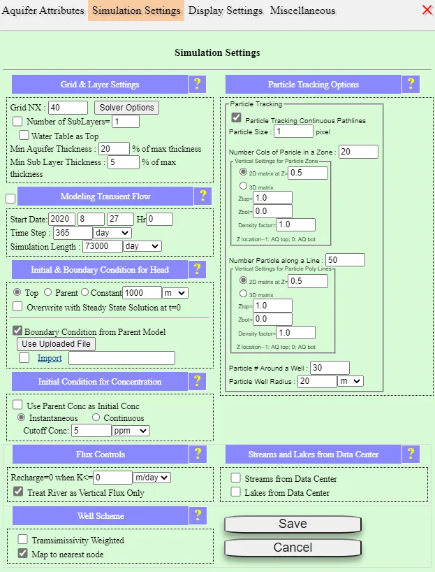
In the Domain Attributes dialog, click the Simulation Settings tab. This tab holds grid, time-stepping, and solver options.
7.2.2 What the fields mean
| Field | Default | What it controls |
|---|---|---|
| Grid NX | 40 | Number of cells along the longer axis of the domain. The shorter axis is sized proportionally to make cells roughly square. Higher NX = finer resolution = slower simulation. |
| Number of SubLayers | 1 | Vertical subdivisions of each conceptual layer. SubLayers = 1 means a 2D solution; SubLayers > 1 resolves vertical gradients. |
| Water Table as Top | Off | Whether to use the computed water table as the top of the aquifer (convertible layers) rather than the DEM surface. Useful when the water table is significantly below the land surface. |
| Total Simulation Time | — (steady) | For transient runs only. Total simulated time in days (or configured units). |
| Time Step Size | — (steady) | For transient runs. Either a fixed step size or an automatic adaptive scheme. |
| Solver | Default | Which numerical solver to use. "Default" picks an appropriate choice based on the engine; options include PCG, SIP, SOR, and Hybrid SOR. |
| Convergence Tolerance | — (engine default) | How tight the head-residual convergence must be. Rarely adjusted; relax only if convergence fails narrowly. |
| BC from Parent Model | Off | For submodels only. Turns on inheritance of boundary conditions from a parent's head solution. |
7.2.3 The solver options
| Solver | Best for | Notes |
|---|---|---|
| Default / Hybrid SOR | Most problems — the platform picks appropriately | Combines the robustness of SOR with the speed of PCG where possible. This is your default. |
| PCG (Preconditioned Conjugate Gradient) | Large problems, MODFLOW-family engines | Fast convergence for well-conditioned problems; the MODFLOW default. |
| SIP (Strongly Implicit Procedure) | Older MODFLOW models, occasional legacy use | Robust but slower. Rarely the best choice for a new model. |
| SOR (Successive Over-Relaxation) | Small problems, educational use, diagnostic runs | Simple but slow. Useful when you want a solver whose behavior is easy to reason about. |
The default solver choice has been engineered to work across virtually all IGW-NET models. Change it only if you have a specific reason — e.g., you're matching a legacy MODFLOW model that used SIP, or you're diagnosing convergence issues and want to test whether a different solver helps. For production work, stick with the default.
7.3 Grid Resolution
Grid NX controls how coarsely or finely your conceptual model (xyz) is approximated by the numerical model (ijk). It is the single setting that most directly trades simulation speed for spatial detail — and deciding when to raise it, when to add sublayers, and when to use a submodel instead is one of the highest-leverage skills in IGW-NET. Each of these choices is ultimately the same question: where does the ijk approximation need to be faithful to the xyz reality, and where can a coarser approximation suffice?
7.3.1 How Grid NX works
NX is the number of cells along the longer side of your domain's bounding rectangle. For a domain that is 20 km × 10 km and NX = 40, the solver uses a 40 × 20 grid of 500 m × 500 m cells. Doubling NX to 80 produces 250 m × 250 m cells — roughly 4× as many cells overall, so simulation time roughly quadruples.
| Domain size | NX = 20 (coarse) | NX = 40 (default) | NX = 80 (fine) | NX = 160 (very fine) |
|---|---|---|---|---|
| 5 km × 5 km | 250 m cells | 125 m cells | 63 m cells | 31 m cells |
| 20 km × 20 km | 1000 m cells | 500 m cells | 250 m cells | 125 m cells |
| 100 km × 100 km | 5000 m cells | 2500 m cells | 1250 m cells | 625 m cells |
7.3.2 The "more resolution is always better" trap
A common instinct — especially among novices, students, and even experienced practitioners coming from other platforms — is that cranking NX higher produces a better model. Push NX to 200, 300, 500 — surely that gives a more accurate answer? This instinct is mostly wrong, and acting on it causes more real problems than almost any other grid-resolution decision.
What actually happens when you raise NX aggressively:
- Compute cost grows super-linearly. Doubling NX quadruples the cell count (2D) or octuples it (3D with sublayers), but simulation time often grows faster than that because solver iterations multiply. An NX = 300 run can be 10× slower than NX = 150, not 4×.
- Convergence deteriorates. Larger linear systems are more ill-conditioned. What converged cleanly at NX = 80 may iterate sluggishly at NX = 160 and may not converge at all at NX = 300. Adding resolution worsens numerical stability beyond a point.
- You may get nothing at all. A failed simulation returns no result — unlike the hope that "at least it'll be a fine-resolution answer," a brute-force attempt that doesn't converge leaves you with neither fine nor coarse. A converged coarse model beats a failed fine one every time.
- Most of the fine resolution is wasted. In a large domain, the features that actually need fine resolution typically occupy a small fraction of the area. Uniformly raising NX over the whole domain is paying fine-grid compute cost for regions where coarse cells would have been perfectly adequate.
Practical NX ceilings for a single simulation in IGW-NET are typically in the 100–150 range — sometimes less. Staying within that range keeps each individual simulation well-posed: fast convergence, robust solver behavior, quick iteration when you're tuning parameters. When you need finer resolution in specific areas, don't push NX higher — use a submodel (Ch. 13). A nested hierarchy gives arbitrary local resolution while keeping every individual simulation well within the convergence-friendly range. The mental shift is from "crank NX up to resolve detail" to "use hierarchy to place detail where it matters." Every level of the hierarchy is well-posed numerically; together they span as much scale range as you need.
This connects directly to Ch. 13 §13.5.1's four-dimension argument for hierarchy. The same reasoning that makes hierarchical models better for cognition, management, and infrastructure also makes them better numerically — a hierarchy of well-posed small problems is easier to solve, debug, and iterate than one big problem at the edge of numerical stability. "More resolution" is not the answer; "hierarchical resolution" is.
7.3.3 When to raise NX
- When cells are obviously too large to resolve features of interest (e.g., a 1 km river on a 2.5 km grid).
- When pumping wells, point sources, or sharp features produce visibly "blocky" results in the head field.
- When convergence is fine but the physics being simulated has scales smaller than the grid can see.
- But — before raising NX, ask whether the detail you need is uniform across the domain (raise NX) or localized (use a submodel instead; see §7.3.4).
7.3.4 When NOT to raise NX (use submodels instead)
If you only need fine resolution in a specific subarea, raising NX on the whole parent is wasteful. A 100 km × 100 km domain at NX = 160 has 25,600 cells; most of those cells are in regions where coarser resolution would be perfectly adequate. The submodel approach — parent at NX = 40, submodel covering the area of interest at NX = 80 or higher — gives you the same local detail for a fraction of the computational cost and keeps each individual simulation well-posed (§7.3.2).
Raise parent NX only when you need finer resolution everywhere. For localized detail, use a submodel. A 20 km × 20 km parent at NX = 40 plus a 2 km × 2 km submodel at NX = 80 gives you 2000 m default resolution region-wide and 25 m resolution locally — for less total compute than raising the parent to NX = 200. This is the standard workflow for site-specific studies embedded in regional context.
7.4 Sublayers and Vertical Discretization
IGW-NET's default 2D solution (1 sublayer) handles most regional and site-scale flow problems. For cases where vertical variation matters, sublayers turn a conceptual layer into a fully 3D computational stack.
7.4.1 What sublayers do
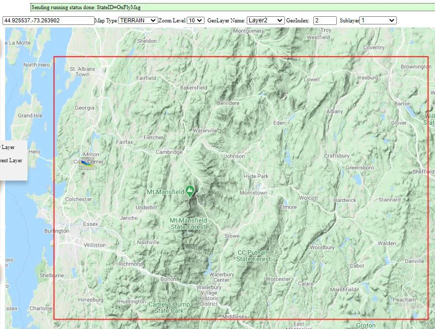
A sublayer value of N means each conceptual layer is subdivided into N computational layers in the vertical. The solver then computes heads, flows, and concentrations in all three dimensions — including vertical head gradients, downward seepage, upward discharge, and vertical plume migration. How the subdivision is positioned vertically matters as much as the number — see §7.4.3 below for the water-table-as-top approach that keeps the subdivision numerically well-posed.
7.4.2 When to increase sublayers
| Modeling situation | Sublayers | Why |
|---|---|---|
| Regional 2D flow, no pumping details | 1 (default) | Vertical resolution provides no benefit when horizontal flow dominates. |
| Pumping wells with partial screens | 3-5 | Captures vertical head gradient near wells; distinguishes what the well actually pumps from. |
| Leaky rivers with bed-aquifer exchange | 3-5 | Vertical flow component between stream bed and aquifer matters for accurate flux calculations. |
| Thick aquifers with K varying vertically | 5-10 | Vertical K heterogeneity has no effect in 2D. With sublayers, each vertical slice can have its own K. |
| Contamination plumes with depth variation | 10+ | Dense or buoyant plumes (DNAPLs, thermal) migrate vertically; resolving this needs fine vertical resolution. |
| Density-dependent flow (SEAWAT) | 10-20 | Saltwater-freshwater interfaces are sharp vertically; fine resolution is essential. |
| Companion to horizontal refinement in submodels | 3-10 (match the study) | When horizontal refinement in a submodel (Ch. 13) captures more local detail, vertical refinement often needs to follow — especially for depth-specific receptors, partial-penetration wells, or vertical plume structure. |
If you're refining horizontally (via a submodel — Ch. 13), you're almost always doing it because local detail matters. Local detail is usually also vertical — a partial-penetration well has depth-specific capture, a contaminant source releases at a specific depth, a stream discharges to specific aquifer horizons. It is rare that horizontal refinement alone is sufficient; vertical refinement via sublayers typically accompanies it. Plan them together when you design a submodel.
7.4.3 How sublayers are positioned vertically — and why water table as top matters
When you set Number of SubLayers = N, IGW-NET subdivides each conceptual layer into N computational layers. But there is a crucial question this raises: what defines the top elevation of the uppermost sublayer? The answer matters enormously for numerical stability and for getting a defensible 3D solution.
Why conceptual layers exist in the first place
Before discussing how to subdivide, a reminder of what a conceptual layer is. Conceptual layers in IGW-NET are chosen to follow major geological units in the xyz reality. A typical regional model of unconsolidated sediments overlying bedrock has one conceptual layer: the unconsolidated aquifer. The conceptual bottom is the bedrock top (from the Data Center or a site-specific raster). The conceptual top defaults to the DEM — the land surface — because for an unconfined aquifer there's no formal upper geological boundary; the aquifer extends up to the water table, which itself sits somewhere below the DEM.
Multiple conceptual layers are used when the geology genuinely has multiple distinct hydrogeologic units — e.g., an upper unconfined aquifer, an intermediate aquitard, and a deep confined aquifer. Each conceptual layer has its own top, bottom, and attributes. Sublayers then subdivide each of those conceptual layers for finer vertical resolution within each geological unit.
The naive approach — subdividing with DEM as the top
The straightforward interpretation of "subdivide the conceptual layer into N sublayers" is to divide the gap between the DEM (top) and the bedrock top (bottom) into N equal parts. This seems obvious, and it is what many simpler platforms do. But it produces a serious problem for unconfined aquifers:
- The DEM has local microtopography everywhere. Small pits, mounds, gullies, buildings, and measurement noise produce rapid up-and-down variation at the sub-10-meter scale. The DEM is the land surface, not the top of the saturated aquifer.
- The real top of the saturated zone is the water table, which is a smooth surface sitting 1–20 meters below the DEM on average, not tracking the DEM's microtopography.
- Subdividing with DEM as top produces chaotic sublayer thicknesses. Where the DEM dips into a small valley, the uppermost sublayer becomes very thin; where the DEM rises on a mound, it becomes thick. Adjacent cells in the upper sublayer can have thicknesses differing by 10× or more.
- This produces dry cells. The uppermost sublayer is above the water table in most places (since the DEM is above the water table). A "cell" above the water table has no saturated thickness — it's dry. The solver handles dry cells, but poorly: iterations multiply, convergence degrades, results become unreliable. On a coarse NX it might work; on finer NX with many sublayers, you get a numerical disaster.
The underlying problem — unconfined flow is nonlinear
The water-table question is not a minor inconvenience. It is a manifestation of one of the well-known hard problems in computational groundwater modeling: unconfined flow is a nonlinear free-surface problem. The top of the saturated aquifer — the water table — is itself an unknown that depends on the solution. Flow equations are written for saturated conditions; the elevation of the saturated zone is what the flow field determines; but solving the flow field requires knowing where the saturated zone is. This circular dependence makes unconfined flow a nonlinear problem that no amount of standard linear-solver sophistication resolves on its own.
The traditional approach in conventional modeling platforms is a fully nonlinear coupled iteration within each simulation: guess a water table, build the cell geometry based on that guess, solve the flow field, update the water table from the result, rebuild cell geometry, solve again, repeat until both the water table and the head field simultaneously converge. This works in principle but is fragile and slow. Each outer iteration rebuilds the grid, introduces step-wise changes to cell thicknesses (cells near the water table can suddenly appear or disappear — the "re-wetting" and "de-wetting" problem), and destabilizes the inner linear solve. Convergence failures are common, especially with many cells, sharp gradients, or thin unconfined layers. Users of traditional platforms know the symptoms: solutions that take forever, diverge entirely, or converge to different answers depending on starting conditions.
The IGW-NET approach — linearize within, iterate between
IGW-NET takes a different approach: linearize the problem within each individual simulation, and iterate between simulations. The mechanism is the Water Table as Top flag combined with the exchange field — IGW-NET's internal mechanism for carrying state between successive simulations.
Within each simulation, the top of the uppermost sublayer is fixed — taken from the previous simulation's head field via the exchange field. With a fixed top, the sublayer geometry is fully determined before the solver runs: every cell has a known thickness, every cell is guaranteed saturated, no re-wetting/de-wetting can happen mid-solve. The flow equations become a clean linear problem — the kind that standard solvers handle in seconds with robust convergence. No nonlinear outer loop is needed inside the simulation.
The nonlinearity doesn't disappear, but it moves outside the simulation: each simulation produces an updated head field; if that updated water table differs meaningfully from the top elevation that was used, you re-simulate with the new head as the new top. This outer loop converges very quickly because the 2D-to-3D correction is usually small — the water table the 2D solve produces is already a good approximation, and the 3D correction is a modest perturbation rather than a dramatic restructuring. One or two iterations typically suffice; convergence of the outer loop is essentially free compared to solving the nonlinear problem monolithically.
This is a well-studied general strategy: transform a hard nonlinear problem into a sequence of easy linear problems that converge to the nonlinear solution. The individual linear solves are fast and robust. The outer iteration is simple to implement and easy to monitor. IGW-NET's implementation — handling all of this behind the Water Table as Top flag and the exchange field — makes it effectively invisible to the user. You check a box, simulate, look at the answer, and if needed simulate again. The platform does the bookkeeping of "use the most recent head field as the new top" automatically.
For users coming from other platforms, this is often the difference between "3D unconfined modeling is painful and frequently fails" and "3D unconfined modeling just works." The underlying problem is the same; the way IGW-NET handles it eliminates the fragility.
The practical workflow
First simulation — 2D (1 sublayer)
Run an initial simulation with SubLayers = 1 (effectively 2D). At this resolution, the head field is the water table — by definition, because with one vertical cell per conceptual layer there is no vertical gradient, so the cell's head equals the water-table elevation at that location. This head/water-table field is what IGW-NET stores as the exchange field for subsequent 3D runs. Getting a good 2D solution is the prerequisite for any 3D elaboration.
Enable Water Table as Top and raise sublayers
In Simulation Settings, check Water Table as Top and raise SubLayers to the desired number (typically 3 for moderate 3D detail, 5–10 for more refined work). Re-SIMULATE. The platform uses the previous 2D head field as the top elevation of the uppermost sublayer, subdivides from there down to the conceptual bottom, and solves the 3D flow on the new sublayered grid — as a linear problem, because the top is now fixed.
(Optional) Iterate once or twice
The 3D solution produces a slightly updated head field (because the 3D solve accounts for vertical flow components the 2D solve did not). If you care about precise water-table elevations — for dewatering, seepage, or wellfield capture work — re-SIMULATE with Water Table as Top still checked; the platform automatically uses the most recent head field as the new top. Typically 1–2 outer iterations are sufficient; the water table converges quickly because the 3D-to-2D correction is a small perturbation.
With water table as top, every sublayer is fully saturated. The linear system is well-conditioned. Each simulation converges as fast as the initial 2D run — often in seconds. There are no dry cells to destabilize the iteration. Adding vertical resolution does not destroy numerical robustness the way it would with naive DEM-as-top subdivision. This is one of the places where IGW-NET's thoughtful default design substantially improves what you get — not just convenience, but the difference between a working 3D simulation and one that fails in confusing ways.
When to skip water table as top
One case where you don't use Water Table as Top: deeply confined aquifers, where the conceptual layer's top is a confining unit (not the land surface) and the aquifer is always fully saturated under pressure. In that case the conceptual layer's top is already a physically-defined elevation (the bottom of the overlying aquitard or confining unit), and subdividing directly produces well-posed sublayers without water-table iteration. For such cases, Water Table as Top should be off.
For everything else — shallow unconfined aquifers, regional unconsolidated-sediment systems, most site-scale studies — Water Table as Top is the right default once you move from 1 sublayer to more.
Going from 1 to 5 sublayers roughly 5× the computational work for a 3D solver. Combined with raising NX, this can quickly make a simulation slow. A good rule: raise sublayers only where physical reasoning justifies it, and verify that the added detail changes the answer before making it permanent. If results with 5 sublayers look the same as with 1, the simpler model is preferable.
7.5 Transient Simulation
Steady-state simulation answers the question "what is the long-term flow pattern?" Transient simulation answers "how does the system respond to changes over time?" The setup is slightly more involved but follows a predictable pattern.
7.5.1 The transient workflow
Run steady-state first
A transient simulation needs an initial condition — the state of the system at t = 0. The easiest (and usually correct) choice is a steady-state solution. Run steady first and let it converge.
Enable transient mode
In Simulation Settings, switch to transient mode. Set the total simulation time (e.g., 1825 days for a 5-year run) and time-stepping parameters.
Configure transient stresses
Identify what changes over time — a pumping rate starting at year 2, a transient head boundary from a stream gauge, a time-varying recharge from a climate file. For wells, use the time-varying rate option. For boundaries, use Head from Transient File. For recharge, use a time-series recharge file.
Simulate
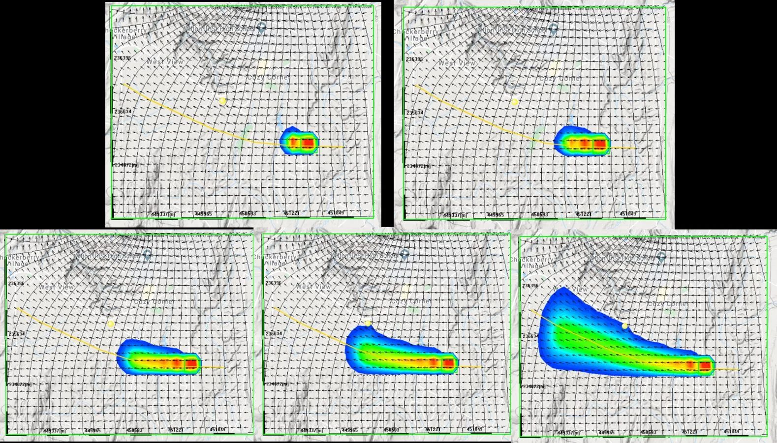
Click SIMULATE. Results stream as an animated movie — head contours, plumes, and particles all evolve in real time as the solver advances through time steps.
7.5.2 The "never accumulate" architecture
As Chapter 1 §1.3.6 noted, IGW-NET operates on one architectural principle across transient flow, Monte Carlo, particle tracking, and transport: simulate, analyze, visualize, discard. Running statistics — mean fields, variance maps, cumulative fluxes, exceedance probabilities — are updated on the fly as each time step or realization completes; the underlying snapshot is then discarded. Memory usage stays constant regardless of how long or how deep the simulation runs.
This is not a clever optimization. It is the only architecture that lets a cloud-native service handle serious modeling — long-horizon transient simulations, probabilistic capture-zone analyses that need hundreds of realizations to converge, high-resolution particle tracking over decades. Platforms that accumulate snapshots in memory hit limits quickly and compromise by running shortened simulations, fewer realizations, or coarser resolution. IGW-NET refuses that trade by never accumulating the data in the first place.
You can run a 100-year transient simulation in a browser without hitting memory limits. What you get is live-streaming statistics (current head field, running mean, running variance, current time step visible) plus any specific snapshots you choose to save. What you don't get (by default) is every time step stored for later replay — if you need that, enable time-snapshot saving explicitly. For most transient analyses, the live-streaming view plus a few saved snapshots is exactly what's needed.
7.5.3 When to save time snapshots
- When producing figures for a publication — you need specific time snapshots (e.g., year 1, year 5, year 10) preserved exactly.
- When doing frame-by-frame video analysis of plume migration.
- When you plan to re-analyze the simulation with different post-processing without rerunning.
For exploratory work, live streaming with running statistics is the faster path. For archival work, saving snapshots at key times is the right choice.
7.6 When Things Go Wrong
The base model is designed to always converge. When it doesn't, something specific in your refinement has introduced numerical difficulty. Here are the common failure modes and how to diagnose them.
7.6.1 Dry cells
A dry cell is a grid cell where the computed head has fallen below the aquifer bottom — meaning the aquifer thickness at that cell is zero. Dry cells have zero transmissivity, so the solver can't move water through them, and nearby heads can swing wildly.
Common causes:
- Bedrock raster too close to surface. If you switched the aquifer bottom from the default constant to a Data Center bedrock raster, and the bedrock rises to near-surface somewhere in the domain, those cells are thin enough that local drawdown dries them out. Fix: revert to the constant bottom, or add a minimum-thickness floor.
- Very low K locally. A zone with K set very low can produce huge drawdowns at any pumping well nearby. Fix: check K values in zones, look for values that are orders of magnitude lower than neighbors.
- Pumping rate too high. A well pumping at an unsustainable rate for the local K and aquifer thickness will eventually dry out its cells. Fix: reduce pumping, or check that Q is correctly specified (in m³/day, with correct sign).
7.6.2 Non-convergence with no clear cause
If the solver reports non-convergence but there are no obvious dry cells or extreme gradients:
- Re-run the base model. Revert your recent refinements to the base model — if it converges, your refinement introduced the issue. Re-apply changes one at a time to isolate which one.
- Relax convergence tolerance. If the residual is just above threshold, loosening tolerance is a pragmatic fix. Be honest with yourself: a loosely-converged solution is approximate, and you should note this when using results.
- Check for features near boundaries. A well too close to a no-flow boundary, or a polyline that straddles it, can create local numerical difficulty.
- Check the projection. In rare cases, an inappropriate projection for a very large domain can introduce numerical issues. Re-accept the default UTM suggestion.
7.6.3 Slow simulation
If simulation is taking noticeably longer than expected:
- Grid NX may be higher than necessary. Reduce for exploration, raise again for final runs.
- Sublayers may be too many for the problem. Use 1 for 2D studies, 3-5 for most 3D needs.
- The domain may be too large for the question. Consider a smaller domain with a submodel for detail.
- Network issues may be slowing streaming. Usually transient; try again.
When something goes wrong, resist the urge to make multiple fixes at once. Change one thing, re-simulate, see if it helped. This is how you actually learn what your model is sensitive to — and how you avoid the situation where "something worked but I don't know what." The real-time visualization makes this kind of disciplined debugging fast, because each iteration takes seconds rather than minutes.
To go deeper
- Chapter 8 — Interpreting the Results — next chapter. Once the simulation converges, this covers how to read what it's telling you.
- Chapter 9 — Transient Simulation — deeper coverage of time-dependent modeling.
- Chapter 10 — Vertical Layering — multi-layer models beyond sublayers.
- Chapter 13 — Nested Modeling — the submodel workflow for localized refinement.
- Platform Concept: The "Never Accumulate" Architecture — how IGW-NET keeps memory constant for long transient and Monte Carlo runs, and why this is the only workable design for cloud-native serious modeling.
- Quick Tutorial 4: Transient Simulation — hands-on walkthrough.