The quick read — 90 seconds
- Transient simulation is for questions about how the groundwater system changes over time — seasonal pumping variations, drawdown recovery, plume arrival times, climate-driven shifts. For long-term averages, use steady-state instead.
- Every transient simulation needs an initial condition — the head field at t = 0. Almost always, this is a steady-state solution from the same model, run first. IGW-NET stores the steady result and uses it as the starting point when you switch to transient mode.
- The time step should match the fastest stress you care about — 30-90 days for seasonal pumping, days-to-weeks for drawdown after a new well turns on, years for long-term climate effects. Platform default: 365 days with 200 steps (good for regional decadal simulations).
- Three kinds of transient stresses: time-varying pumping/injection rates at wells, time-varying boundary heads via CSV files (Type 8 polylines), and time-varying recharge from a file. Each is configured separately.
- IGW-NET's never-accumulate architecture applies to time as well as realizations: simulate, analyze, visualize, discard. Memory stays constant regardless of simulation length. Enable snapshot saving explicitly for time steps you want preserved.
- Transient results are movies, not photos. You watch heads evolve, plumes migrate, particles animate — in real time as the solver advances. Hydrographs at monitoring wells and breakthrough curves are where quantitative interpretation happens.
9.1 When Transient Matters
The first question to ask before setting up a transient run is whether you actually need one. Transient simulations take longer, require more configuration, and introduce more places things can go wrong. For many groundwater questions, a steady-state solution is both sufficient and preferable.
9.1.1 Questions steady-state answers well
If your question fits one of these patterns, steady-state is almost always enough:
- "What is the long-term average flow pattern?" Regional flow systems, baseflow distribution, general groundwater circulation.
- "Where does water that enters here eventually discharge?" Steady-state flow fields with particle tracking answer this without needing time.
- "What is the capture zone of a well pumping at a constant rate for decades?" After a few years, a constant-rate capture zone stabilizes — steady-state gives you the stabilized shape.
- "What is the average baseflow this river receives?" Steady-state computes the long-run discharge; year-to-year variation usually averages out at the scales most watersheds care about.
- "Is my conceptual model even right?" For calibration against average conditions — which is how most regional calibration works — steady-state gets you there faster.
9.1.2 Questions that require transient
Transient simulation becomes necessary when time is part of the answer — when "when" or "how long" is the question, not just "where" or "how much":
| Question | Why transient is needed |
|---|---|
| "How long until the plume reaches the water-supply well?" | Arrival time is intrinsically a transient question — the answer is a date, not a location. |
| "What is the drawdown response to a new pumping well?" | Drawdown develops over days-to-years; transient resolves the response curve. |
| "How do heads vary seasonally?" | Steady-state gives one answer; the real system has seasonal highs and lows driven by recharge cycles and pumping schedules. |
| "If we stop pumping, how fast does the aquifer recover?" | Recovery is transient by definition. Steady-state would give the eventual recovered state but not the timeline. |
| "How does contaminant concentration at my monitoring well change over the next 20 years?" | Breakthrough curves are transient objects; steady-state gives only the eventual plateau. |
| "What is the effect of a changing climate (wetter / drier / different seasonal distribution)?" | Climate effects manifest in time-varying recharge; transient resolves the aquifer's delayed response. |
| "Does an aquifer test support my estimate of transmissivity and storage?" | Aquifer tests are fundamentally transient — transmissivity governs steady response, storage governs transient response. Steady-state can't even see storage. |
A quick diagnostic. Steady-state ignores storage entirely — specific yield and specific storage don't enter the equations. If the answer to your question depends on how much water the aquifer can release per unit head change, you need transient. If it doesn't, you don't. Pumping response, drawdown recovery, seasonal cycles, aquifer tests — all storage-sensitive. Long-term average flow patterns, general plume direction, capture-zone shape — not storage-sensitive.
9.1.3 When to start with steady and add transient later
Even when you know you'll need transient results, start with steady-state. Three reasons:
- Debugging is easier. A steady-state run surfaces structural problems (bad parameters, misconfigured features, domain issues) without the confounder of time-stepping complications.
- The steady result becomes your initial condition. You cannot run transient without one, and steady-state is almost always the right choice.
- Calibration is usually steady-first. Match average heads in steady-state, then refine storage parameters in transient to match hydrographs. Trying to do both at once has too many moving parts.
This chapter assumes you have a converged steady-state model. If you don't yet, go back to Chapter 7 and get one before continuing here.
9.2 The Steady-to-Transient Workflow
Turning a steady model into a transient one is a three-step operation: flip the simulation mode, tell the platform to use the steady result as the initial condition, and configure any stresses that change over time. Every step has sensible defaults, so a first transient run is usually fast.
9.2.1 Step by step
Start from a converged steady-state solution
Run your steady-state model, verify it converges (Ch. 7 §7.6), check the water balance closes (Ch. 8 §8.4). Do not proceed to transient until the steady solution is clean. Problems left in the steady model will compound in transient.
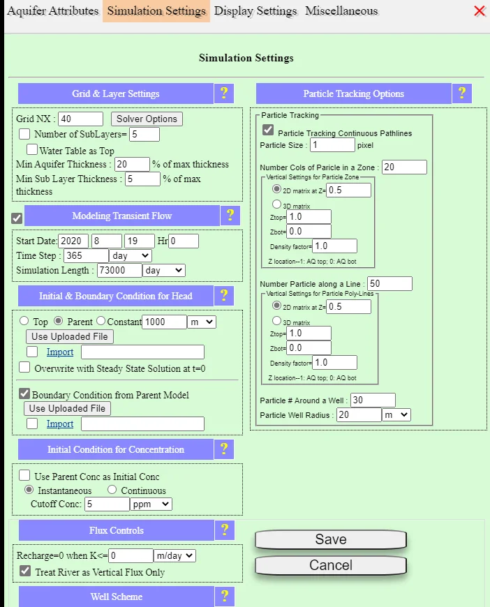
Open Simulation Settings
Click DomainAttr and switch to the Simulation Settings tab.
Enable transient mode
Check Modeling Transient Flow (or equivalent label). Additional fields become visible: total simulation length, time-step size, initial-condition source.
Choose the initial condition
Select Use previous steady solution as initial condition. This is almost always what you want. Alternatives (uniform head, imported field) exist for specialized cases.
Set simulation length and time step
Total simulation time defaults to 73,000 days (200 years) with 365-day (1-year) steps — a good starting point for regional decadal questions. Adjust for your problem (see §9.3).
Configure transient stresses
If any of your wells, boundaries, or recharge inputs change over time, enable their transient options (§9.4, §9.5, §9.6). If nothing changes, you'll get a transient run with constant stresses — useful for showing how the system reaches steady-state, but not usually what you want.
Simulate
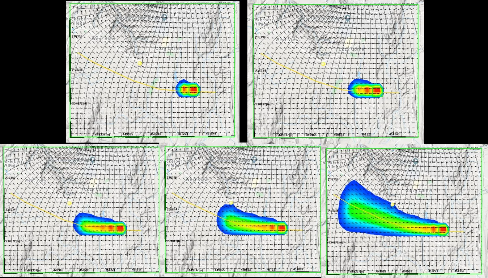
Click SIMULATE. The solver starts from the steady initial heads and advances step by step. Results stream as an animated movie — heads, plumes, and particles all evolve in real time.
9.2.2 Why the steady initial condition matters so much
If you skip the steady initial condition and try to start transient from scratch, the first several time steps spend themselves just reaching a plausible flow field. The early-time results aren't physically meaningful; they're transient artifacts of the solver's struggle to converge to reasonable heads. By contrast, starting from a converged steady solution means the very first time step is already a physically plausible state — you see the system responding to transient stresses immediately, not recovering from an arbitrary starting point.
There are rare cases where steady-state is the wrong initial condition: aquifers that are not actually in steady-state at the start of your simulation period (a newly filled reservoir, a recent large land-use change, an aquifer recovering from historical over-pumping). In those cases you may need a spin-up — run a longer transient simulation that starts from an approximate state and lets the system naturally reach the "initial" conditions you care about, then use that as the true start of your analysis. This is uncommon but worth knowing about. For most systems, the steady assumption at t = 0 is defensible.
9.3 Choosing the Time Step
Time-step size is the single most consequential numerical choice in transient modeling. Too small wastes computation; too large smears out the time behavior you are trying to see. The general rule is simple — match the step to the fastest stress you need to resolve — but the practical choices depend on what question you're asking.
9.3.1 Recommended time steps by problem type
| What you're simulating | Time step | Total length | Steps |
|---|---|---|---|
| Aquifer test (minutes-to-days) | 1 minute to 1 hour | 1-10 days | ~200-1000 |
| Short-term dewatering, construction pumping | 1-7 days | 30-365 days | ~30-200 |
| Seasonal pumping and recharge cycles | 30-90 days (monthly to seasonal) | 2-10 years | ~20-100 |
| Drawdown recovery after new well startup | Daily at start, stretching to monthly/yearly | 5-50 years | ~50-200 (adaptive) |
| Plume migration at a site | 30-365 days depending on flow velocity | 10-100 years | ~30-200 |
| Regional decadal response (climate, land use) | 365 days (1 year) | 50-200 years | ~50-200 (platform default) |
| Long-term evolution (aquifer depletion, geological) | 1-10 years | 100-1000+ years | ~100-200 |
9.3.2 The platform default, explained
IGW-NET's default transient run is 73,000 days (200 years) with a 365-day time step — giving 200 steps total. This is a deliberately generous default meant for regional decadal-to-century simulations: seeing how a basin responds to pumping changes, climate shifts, or long-term recharge trends. For shorter site-scale questions, reduce both the time step and the total length to fit your problem.
If you're not sure what time step to choose, run the default first. Watch the animation. If heads seem to jump between steps (too large) or nothing visibly changes over many steps (too small), adjust. Because IGW-NET streams results in real time, this adjustment loop is fast — a few iterations usually find the right balance.
9.3.3 Adaptive time stepping
For problems with very different timescales — like rapid drawdown at a new well followed by slow long-term equilibration — a fixed time step is inefficient. Daily steps for 50 years is 18,000 steps, most of them wasted. The solution is adaptive time stepping: short steps at the start when heads are changing fast, gradually lengthening as the system settles toward steady response.
When adaptive stepping is available for your selected engine, enable it via Simulation Settings. Specify a starting step, a growth factor (typically 1.2-1.5 per step), and a maximum step. The solver advances: short steps at first, each slightly longer than the last, until reaching the maximum. This resolves the early transient cleanly and efficiently handles the long tail.
9.4 Transient Pumping Schedules
Most transient groundwater models have at least one stress that changes over time, and most commonly that stress is a pumping schedule. Wells turning on and off, seasonal pumping variations, operations changes — each is a time series of pumping rates applied at a well.
9.4.1 Enabling time-varying pumping
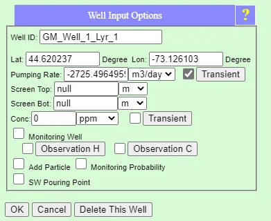
Open the well's attributes
Double-click the well on the map, or select it and open its Input Options dialog.
Enable time-varying rates
Check Enable time-varying pumping/injection (or the platform's equivalent label). The static Q field is replaced by — or supplemented with — a time-rate table.
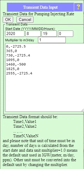
Populate the schedule
Enter (time, Q) pairs. Time is measured from the start of the transient simulation; Q is pumping rate in m³/day with the same sign convention as static wells (negative = extraction, positive = injection). The platform interpolates linearly between pairs. For complex schedules, load from CSV.
Save and simulate
The well now follows the schedule during simulation. Each time step, the solver reads the interpolated Q at that simulation time and applies it.
9.4.2 Common pumping-schedule patterns
| Schedule type | Typical use | How to build it |
|---|---|---|
| Step change | New well starts at a specific date; well taken offline | Two time-rate pairs: (t=0, 0) then (t=startup, Q). Platform interpolates linearly, but the step is sharp enough to be effectively instant. |
| Seasonal cycle | Agricultural pumping, summer water demand | Four-to-twelve pairs per year tracing the annual cycle. Repeat the pattern over the simulation length or use a periodic-function loader. |
| Ramp-up / ramp-down | Gradual expansion or retirement of a well field | Linear interpolation between the start Q and end Q over the transition period — exactly what linear interpolation gives you with two pairs. |
| Historical observations | Calibration against known pumping records | Load from CSV. Time-rate pairs at monthly or quarterly observation intervals, directly from the pumping logs. |
| Stochastic future scenarios | "What if" planning under uncertain future demand | Multiple runs with different schedules; use Monte Carlo framing (Ch. 18) for systematic uncertainty. |
The same rule from Ch. 6 §6.4 applies: negative Q for extraction, positive for injection. A well that alternates — extracting water for supply, then injecting treated water back as part of a remediation loop — enters the schedule with alternating signs. Zero Q is allowed and means the well is inactive for that period.
9.5 Transient Recharge
Recharge is the second most common time-varying stress. Seasonal patterns, year-to-year precipitation variability, multi-decade climate trends — all express themselves through a recharge signal that differs by month, year, or decade.
9.5.1 Three ways to specify transient recharge
IGW-NET handles transient recharge at three levels of detail, matching the customization ladder from Ch. 5 §5.7:
| Method | Spatial | Temporal | Best for |
|---|---|---|---|
| Constant recharge (no transient recharge) | Uniform (or zone overrides) | Constant throughout simulation | Simulations where only pumping or boundary conditions change over time; long-term average climate. |
| Transient recharge time series (uniform spatial) | Uniform across domain | Changes over time | Climate-driven studies where seasonal or interannual precipitation variations matter but spatial variation is secondary. |
| Spatially distributed, temporally varying recharge | Grid or Data Center raster stack | Changes over time, different per cell | Detailed climate or land-use studies where recharge varies both in space and time — the most data-intensive option. |
9.5.2 Enabling a transient recharge time series
For spatially uniform but temporally varying recharge — the most common case — open Domain Attributes, go to the Recharge tab, and enable Time-varying recharge. The table accepts (time, recharge) pairs in units consistent with your domain (typically m/day or inches/year, depending on the platform setting).
Climate-driven patterns to consider:
- Seasonal cycle. High recharge in wet months (spring, autumn), low in dry months (summer, winter where frozen). Twelve pairs per year traces the monthly cycle.
- Interannual variability. Year-to-year wet/dry cycles. Load from historical data if calibrating, or generate from climate projections if forecasting.
- Multi-decade trends. Climate projections showing gradual increases or decreases. Specify as a slow linear ramp or as a realization from a climate model.
9.5.3 Transient recharge with spatial variation
For climate studies that need both spatial and temporal detail, IGW-NET accepts a stack of recharge rasters — one per time interval — loaded from a Data Center service or uploaded. The platform assigns each raster to its corresponding simulation time; recharge at each cell is then the value from the time-appropriate raster.
This is data-intensive — a 10-year monthly simulation needs 120 rasters — and is typically reserved for detailed calibration or climate-impact studies. For most transient work, spatially uniform time-varying recharge is sufficient.
Chapter 5 §5.8.3 established the mass-balance principle: in a regional system, whatever enters as recharge must leave somewhere. In a transient simulation, the "somewhere" and the "when" can be decoupled — recharge in winter may discharge as baseflow in summer, with storage cycling between. This storage effect is exactly what transient models capture that steady-state ones cannot. If you watch a transient simulation of a temperate aquifer, you see the storage fill in wet seasons and drain in dry ones; the annual average matches steady-state, but the monthly behavior is dramatically different.
9.6 Transient Boundary Heads
When a boundary condition itself changes over time — a river whose stage fluctuates seasonally, a reservoir whose level is managed, a regional water table whose historical trend is known — the polyline type 8 · Head from Transient File is what you reach for.
9.6.1 Using Type 8 polylines
Chapter 6 §6.3.2 introduced the nine polyline types. Type 8 is the transient-head option. Drawing a Type 8 polyline follows the same workflow as any other polyline (§6.3.1), with one additional step:
Draw the polyline
Trace the line feature (river, drain, boundary segment) the same way as any other polyline.
Set type to "Head from Transient File"
In the Edit Polyline Attributes dialog, choose Type 8 from the dropdown.
Upload the transient file
Provide a CSV with columns for time and head (optionally with additional columns for per-vertex variation). Time is in simulation-time units; head is in elevation units matching your domain.
Verify interpolation
The platform reads the CSV at each time step and interpolates to the current simulation time. Check a couple of intermediate times (e.g., via a Statistics query during simulation) to confirm the values are what you expected.
9.6.2 Common transient-head sources
- USGS stream gauges. Daily or hourly stage records for rivers. These can be pulled directly via DataNET's USGS bridge or uploaded as CSV.
- Reservoir operations records. Monthly stages from dam-operations logs.
- Tidal signals. For coastal aquifers where sea-level variation matters; periodic functions or tide-gauge data.
- Historical climate reconstructions. Paleo-climate or pre-observational reconstructions used for long-term historical simulations.
- Climate projections. Future-scenario outputs from global or regional climate models, for forecasting simulations.
It's tempting to use the finest-resolution data available — hourly stage records, for instance — but this rarely helps. The aquifer smooths out high-frequency boundary variations over distance, so hourly input at a boundary 500 m away produces negligible difference from daily averaged input. Match boundary-head resolution to your time step and to the relevant timescale of the aquifer's response. For most regional simulations, daily is fine; for most site-scale simulations, monthly is ample.
9.7 "Never Accumulate" — For Time
Chapter 1 §1.3.6 introduced IGW-NET's core architectural principle: simulate, analyze, visualize, discard. For transient simulation, this principle is what makes multi-decade and multi-century runs feasible in a browser.
9.7.1 What gets discarded and what gets kept
During a transient run, each time step produces a complete flow state — heads, concentrations, velocities, particle positions. Storing all of them for a 200-step simulation means storing 200 full-domain snapshots. For a 100,000-cell model with head, concentration, and flow fields, that's gigabytes of data per simulation. For a 500-realization Monte Carlo (Ch. 18), multiply by 500 — approaching a terabyte. No browser can handle that.
IGW-NET's response is to refuse the accumulation:
| Kept (running) | Discarded (per step) |
|---|---|
| Current head, concentration, and flow fields (overwritten each step) | Previous step's full state snapshots |
| Running statistics: mean head, variance, min/max heads, cumulative fluxes, time-integrated quantities | Per-step increments (absorbed into running statistics then discarded) |
| Hydrographs at monitoring wells (one value per well per step) | Non-monitoring cell histories |
| Breakthrough curves at monitoring points (one concentration per point per step) | Non-monitored concentration histories |
| Flux time series across Type-4 polylines | Per-cell flux details |
| Explicitly saved snapshots (if you requested them) | All other time-step snapshots |
9.7.2 Saving snapshots when you need them
The default is never-save; but there are cases where you genuinely need specific time snapshots preserved — for report figures, for frame-by-frame analysis, or for later post-processing. IGW-NET lets you opt in to snapshot saving:
- Specific times. Save at t = 365 days, t = 1825 days (5 years), t = 3650 days (10 years), etc. — the times you'll want for your figures.
- Periodic intervals. Save every N time steps (e.g., every 10th step for animation frames).
- Triggered saving. Save when a condition is met — e.g., when plume concentration at a monitoring well first exceeds the MCL.
Saved snapshots are persisted to your account and can be loaded back for analysis. Use this capability judiciously: each saved snapshot is substantial, and saving many defeats the purpose of the never-accumulate architecture.
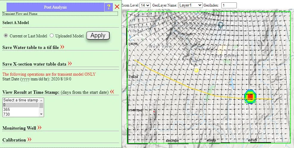
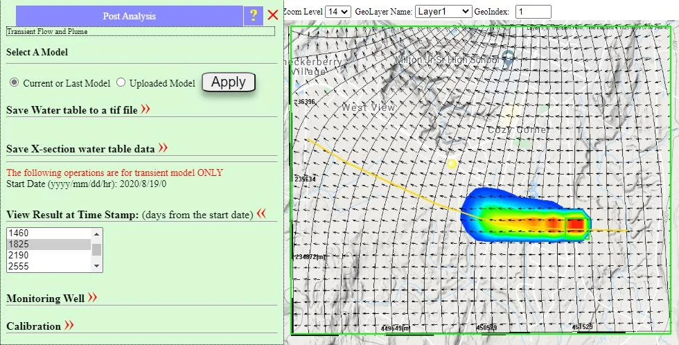
The never-accumulate architecture reflects a specific stance on what modeling is for. If your goal is to produce a large data artifact — a detailed multi-dimensional output to be stored and re-analyzed later — IGW-NET's default behavior is inconvenient. If your goal is to develop understanding — to watch the system respond and build intuition about the processes — never-accumulate is exactly right. The visualization IS the product. What you need after the simulation is the running statistics, the hydrographs at places you care about, and the handful of snapshots that will appear in your report. Everything else was scaffolding for the solver, not the point of the exercise.
9.8 Reading Transient Results
Steady-state results are a photograph. Transient results are a movie, a set of hydrographs, and a handful of saved frames. Interpretation is different — pattern recognition across time, not just across space.
9.8.1 The animated plan view
As each time step completes, the plan view updates — head contours shift, plumes migrate, particles animate along the current flow field. The visual experience is closer to watching a weather map evolve than looking at a static figure.
What to look for:
- Response to stress changes. When a well turns on, does the cone of depression develop gradually and stabilize? When recharge surges in spring, do heads rise regionally and contour spacing tighten near discharge features?
- Plume evolution. Where does the plume go? How fast? Does it hit sensitive receptors, and at what time? Do density effects or sorption alter the trajectory over time?
- Flow-field reversals. In some stressed systems, pumping inversions can cause local flow directions to reverse. Transient visualization shows this; steady-state averages it out.
- Feedback loops. Pumping drops heads, drops heads reduce stream-aquifer exchange, reduced exchange further stresses the aquifer. Watching these feedbacks in real time is revealing.
9.8.2 Hydrographs
A hydrograph at a monitoring well is the quantitative signature of transient response at that location. For each well with isMonitoringWell = 1 (Ch. 6 §6.4), the Analysis Tools produce a time-series chart of head vs simulation time.
Reading a hydrograph:
- Initial value — the steady starting head at that location.
- Rate of change — how fast heads are responding to stresses. Slope gives you the time-scale.
- Seasonal oscillation — annual cycles from recharge and pumping.
- Long-term trend — gradual rise or fall from climate, development, or pumping changes.
- Step changes — abrupt jumps usually indicate a stress change (new well, boundary shift).
- Asymptotic behavior — does the hydrograph approach a new steady value, continue changing indefinitely, or oscillate around an average?
9.8.3 Breakthrough curves
For transport simulations, the concentration-over-time plot at a downgradient monitoring well is a breakthrough curve. It answers questions steady-state cannot:
- Arrival time. When does contamination first show up?
- Time to MCL. When does concentration exceed regulatory thresholds?
- Peak and decay. What is the maximum concentration and when does it decline?
- Tailing. Long, slow concentration declines indicate dispersion, sorption, or dual-domain exchange (Ch. 12).
Breakthrough curves are the foundation of risk analysis. They are also one of the most sensitive outputs to model parameter choices — small changes in K or dispersivity can shift arrival times by years.
9.8.4 Multi-layer transient visualization
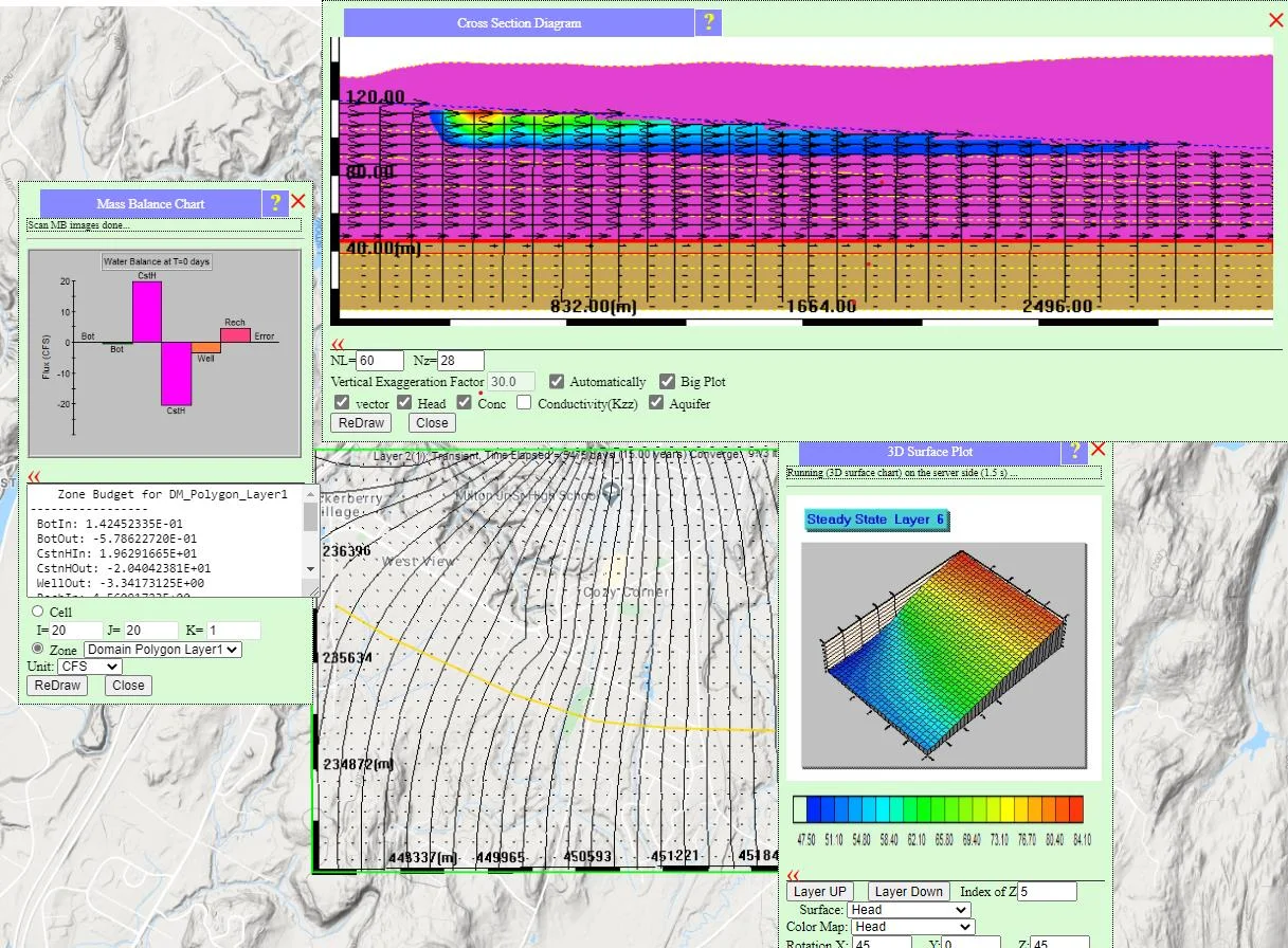
When the model has vertical layers (Ch. 10), cross-sections in transient simulation reveal inter-layer dynamics that 2D cannot capture. Upper-layer heads respond quickly to recharge pulses; lower layers respond more slowly, with a lag set by vertical K and confining-layer storage. The delay between layers is physically meaningful — it's why water wells in confined aquifers often see delayed responses to surface events — and it's visible directly in the transient cross-section animation.
9.8.5 Water balance over time
The water-balance tool (Ch. 8 §8.4) continues to work for transient runs, but now with time as an additional dimension. You can look at:
- Running totals. Cumulative recharge, cumulative pumping, cumulative baseflow over the simulation period.
- Storage change. Unlike steady-state, transient runs have a non-zero storage term — water going into or coming out of aquifer storage. This is the signature time-dependent behavior.
- Time-varying imbalance. Occasionally a transient run will show water-balance errors growing over time; this usually indicates a convergence or time-stepping issue. Investigate rather than accept.
In a steady-state water balance, inflow = outflow and storage change = 0 by definition. In a transient water balance, storage change is usually non-zero. If your transient run shows storage change = 0 at every step, you may have accidentally stayed in steady-state mode. If your storage change is oscillating wildly, you may have a time-step problem (too-large steps creating numerical instability). If your storage change is trending monotonically in one direction, the aquifer is gaining or losing water over the simulation period — meaningful if climate or pumping is changing, suspicious if conditions are stable.
To go deeper
- Chapter 10 — Vertical Layering — next chapter. Transient behavior gets richer when multiple layers interact.
- Chapter 12 — Contaminant Transport — transport is almost always transient; breakthrough curves and plume evolution live there.
- Chapter 17 — Calibration — how to calibrate transient models against observed hydrographs.
- Chapter 18 — Stochastic Modeling — combining transient with Monte Carlo for risk-based prediction.
- Platform Concept: The "Never Accumulate" Architecture — the architectural principle that makes long transient runs feasible.
- Quick Tutorial 7: Transient Modeling — hands-on walkthrough of a pumping-schedule scenario.
- Case Study: Mancelona TCE Plume — a real transient transport simulation with decadal time series.