The quick read — 90 seconds
- A conceptual layer is a real geologic unit (sand aquifer, clay aquitard, bedrock aquifer). A sublayer is a numerical discretization of a single conceptual layer into multiple vertical cells. They serve different purposes and combine: a two-conceptual-layer model with 5 sublayers per layer gives you 10 computational cells vertically across two distinct materials.
- Add conceptual layers when you have real geology to represent — a confining clay unit between aquifers, a deeper bedrock aquifer, a multi-tier aquifer system with different K in each layer.
- Add sublayers when the aquifer is uniform but vertical gradients matter — partially-penetrating wells, DNAPL plumes descending through an aquifer, detailed dispersion studies. Chapter 7 §7.4 covered this.
- Layers communicate vertically via vertical hydraulic conductivity (Kz). Typical aquifers have anisotropy Kh/Kz = 10 to 1000 — vertical flow is much more restricted than horizontal. A confining unit is specifically a layer with very low Kz (10-6 to 10-3 m/day) that drastically restricts vertical exchange.
- Layer elevations (top and bottom of each layer) follow the customization ladder from Chapter 5 — constant, Data Center raster, uploaded raster, scattered points from boreholes, or T-PROGS geostatistical realizations (Ch. 16).
- When in doubt, start 2D. Multi-layer models are harder to build, harder to debug, and slower to simulate. If your question can be answered in 2D, answering it in 3D usually adds cost without adding insight.
10.1 Conceptual Layers vs Sublayers
The single most important distinction in this chapter is the one between conceptual and computational layering. Confusing them leads to over-complicated models that don't do anything useful; understanding them lets you add vertical structure exactly where you need it.
10.1.1 Conceptual layers represent geology
A conceptual layer is a distinct geologic unit with its own set of hydraulic properties — K, porosity, storage, top and bottom elevations. Each conceptual layer represents a physically real piece of the subsurface: a sand aquifer, a clay aquitard, a bedrock aquifer beneath, a glacial-drift layer above. The boundaries between conceptual layers are real geologic contacts; the parameters on each side are different because the materials are different.
In IGW-NET, you set the number of conceptual layers in the model's header and configure each layer's attributes separately. A single conceptual layer is the default — appropriate for most near-surface, unconfined-aquifer modeling. Two or three conceptual layers represent common stacked systems (surficial aquifer + confining unit + deep aquifer). More than three is unusual outside of specialized contexts like layered sedimentary basins.
10.1.2 Sublayers resolve vertical gradients
A sublayer is a numerical subdivision within a single conceptual layer. Sublayers have the same material properties as the conceptual layer they subdivide; they exist solely to resolve vertical variation in head, flow, and concentration within a physically uniform layer.
A conceptual layer with 1 sublayer is computed as a single vertical cell per grid position — the 2D default. A conceptual layer with 5 sublayers is computed as 5 stacked cells; the solver tracks head, flow, and transport separately in each sublayer. Chapter 7 §7.4 covered when to raise the sublayer count.
10.1.3 How they combine
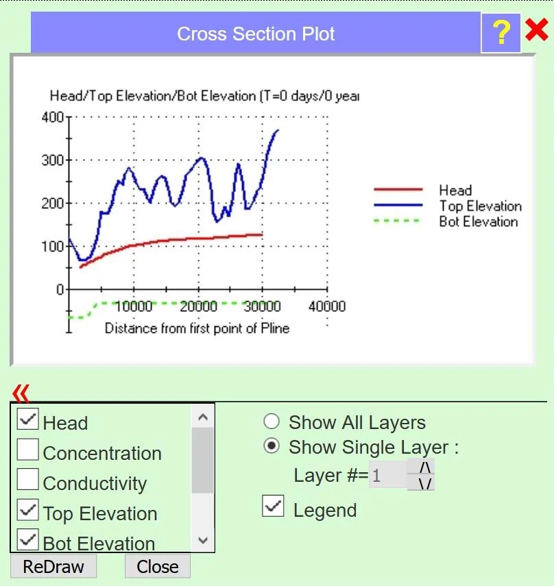
| Configuration | Conceptual × Sublayer | Total cells vertical | Typical use |
|---|---|---|---|
| 2D, single aquifer | 1 × 1 | 1 | Regional near-surface aquifer, most first-model work |
| 2D with vertical resolution | 1 × 5 | 5 | Single-aquifer model with partial wells, DNAPL sinking, or detailed vertical transport |
| Two-layer system | 2 × 1 | 2 | Surficial aquifer above a deeper aquifer with different K, no vertical resolution within each |
| Three-layer with confining unit | 3 × 1 | 3 | Typical "upper aquifer / clay aquitard / lower aquifer" stratigraphy |
| Detailed multi-tier model | 3 × 5 | 15 | Complex stratigraphy with within-layer vertical detail — research or detailed site investigations |
If adding a vertical division changes the material — K, porosity, storage all different on one side vs the other — it's a conceptual layer. If the division just splits an otherwise uniform aquifer into more computational cells, it's a sublayer. Real confining units are always conceptual layers; detailed vertical resolution within a single sandy aquifer is sublayers.
10.2 Deciding to Add Layers
Most IGW-NET models can — and should — stay 2D. Adding vertical layers increases complexity substantially; the decision to do so should be deliberate, driven by a specific question that 2D cannot answer.
10.2.1 Stay 2D when
- You're modeling a near-surface, unconfined aquifer with no meaningful stratigraphy. Most surficial aquifer-water-supply questions fit here.
- The aquifer is thin relative to horizontal extent. If the aquifer is 50 m thick and the domain is 20 km across, horizontal flow dominates and vertical gradients are negligible at regional scales.
- Your question is about long-term average patterns, not detailed vertical distribution. Recharge, baseflow, regional flow direction, wellhead-protection areas — all 2D-friendly.
- You don't have data to constrain a 3D model. Adding layers you can't parameterize adds free parameters without adding predictive power.
10.2.2 Add conceptual layers when
- There is a confining unit separating aquifers. A clay aquitard, a shale bed, a till layer — any laterally-continuous low-K unit that matters for the flow system.
- Different aquifers serve different purposes. A shallow irrigation aquifer above a deep drinking-water aquifer, where contamination risk needs to be evaluated for both.
- You have borehole data showing distinct stratigraphy. If borehole lithology logs consistently show sand over clay over sand, that's a three-layer system.
- Vertical head differences between units matter. If artesian conditions exist in a lower aquifer (heads higher than surface), a 2D model cannot represent this.
- Contamination risk depends on vertical pathway. For contaminants reaching a deep aquifer, the aquitard's integrity is the whole question — a 2D model can't evaluate it.
10.2.3 Add sublayers when
- Partially-penetrating pumping wells — where the well screens only part of the aquifer. A partial well creates vertical head gradients that a 2D model averages away.
- DNAPL or dense plume sinking — where a contaminant is heavier than water and descends through the aquifer. Needs vertical resolution to capture.
- Leakage characterization — detailed study of vertical flow near a leaky river or lake, where the exchange is concentrated in the top portion of the aquifer.
- Density-dependent flow (SEAWAT) — seawater intrusion, where the freshwater-saltwater interface is a vertical feature.
Here's a useful shortcut: if your aquifer is layered but the confining units are thin and you don't care about within-aquifer vertical detail, you can sometimes use a single conceptual layer with effective properties that represent the layered system as a whole — computing a vertically-averaged K that accounts for the layer structure, but modeled as one layer. This is less accurate than explicit layering but often enough for regional questions and vastly simpler. Chapter 5 §5.5 touched on effective K; the same principle applies to effective vertical transmissivity.
IGW-NET supports two complementary ways to model vertical flow dynamics, and the distinction between them matters because each has different physical guarantees.
Approach 1 — Prescribed water table (2D vertical profile). Enter synthetic mode via Utilities → Go to Synthetic Case Area. Treat the y-axis as elevation. Draw a polyline representing the water table shape — sloping, wavy, sinusoidal, stepped — and assign its head via the Equal to Y (e.g., Water Table) prescribed-head option. The solver reads this as head = y along the drawn line, consistent with the physical definition of a water table (pressure = 0, so head = elevation). Mark the region above the water-table line as Inactive so the solver operates only below. Simulate. Classic Tóth regional circulation appears — local, intermediate, and regional flow cells stacked vertically beneath a sloping or wavy water table. Add an internal horizontal layer of higher or lower K (for example, a basal high-K sand unit, or an internal aquitard) and you see what structural geology does: water routes itself through high-K zones, pools above aquitards, and builds "extended Tóth" circulation patterns where geological layering redirects the natural flow pathways from recharge to discharge. The visualization is revealing — you see, quantitatively and vividly, how water self-optimizes its route through the subsurface.
Anisotropy handling. In the vertical profile, horizontal K is typically much larger than vertical K. If you vertically exaggerate the profile display by √(Kx/Kz) the geometry becomes effectively isotropic in the transformed coordinate — which is why hydrogeological cross-sections are conventionally shown that way. The math runs correctly regardless; the exaggeration is a display convention for human readability.
Tutorial: Tutorial 12 — 2D Cross-Sectional Profile Modeling walks through this approach end-to-end, including the basal high-K unit that generates the most pedagogically satisfying circulation patterns.
The prescribed-water-table method is physically correct only when the water table you draw and the aquifer K field you specify are mutually compatible — that is, when the recharge and discharge fluxes implied by the simulated flow field could plausibly be supplied by actual rainfall and actual discharge pathways. When they aren't compatible, the simulation is kinematically valid but physically unrealistic.
Here is why this happens. The solver is asked: "given this water-table shape, what head field and flow field satisfy Darcy's law?" It finds an answer — always, because the problem is well-posed. But the answer implies a total water flux moving through the domain, and there is no constraint tying that flux back to rainfall recharge. If you draw a steeply-sloping water table and assign high K, the solver will happily produce enormous fluxes. The head distribution and flow pattern look beautiful and physically sensible as pictures, but the flux is not a flux that real rainfall could ever produce. A pedagogical Tóth system might move water through the subsurface at rates one or two orders of magnitude above what the overlying climate could supply — a flagrant violation of the water balance.
This matters pedagogically. When you show students a Tóth circulation pattern from a prescribed water table, tell them: the geometry of flow is real; the magnitude of flow is only as realistic as the compatibility between the water table you drew and the K field you assigned. A useful check: compute the total discharge flux from the simulation and compare it against the area of the domain times a realistic recharge rate. If the simulated flux is more than ~2× this upper bound, the prescribed water table is too steep for the K you specified, or the K is too high for the water table shape.
Fix: either reduce K, flatten the water table, or switch to Approach 2 below.
A rigorous alternative: build a 3D model that is one cell wide in the plan view (a narrow "slice") but fully resolved vertically. In plan view this is a one-cell-wide strip; in vertical elevation it has one or more geological layers, each subdivided into many computational sublayers (Ch. 10 §10.1). The top boundary is the DEM (real topography, in georeferenced mode) or a user-defined top (in synthetic mode). Recharge is applied as an infiltration flux at the top. The water table then emerges as part of the solution — you do not prescribe it. The solver finds the water-table elevation that is consistent with the specified recharge flux, the aquifer K field, and the boundary conditions. By construction, the flux moving through the system equals the recharge you supplied, so the water balance is guaranteed.
In georeferenced mode, this approach is especially revealing when applied to a real landscape. A slice 3D model through glaciated Michigan terrain, using the DEM as the top and realistic recharge (say ~10 inches per year) as the input, produces a vertical profile whose water table respects the real topography, whose fluxes are compatible with the rainfall, and whose internal circulation reflects both the terrain and the hydrostratigraphy. What you see is not a clean Tóth idealization but something closer to the real complexity of glaciated aquifers — shallow flow cells pinned to topographic highs and lows, deeper regional flow where the hydrostratigraphy permits, and confining-layer effects where they exist. The picture is messier than the prescribed-water-table idealization, but it is the picture you can trust.
When to use each approach. Use prescribed-water-table (Approach 1) when the goal is to visualize the geometry of regional-flow circulation for teaching, or when you have an independently-known water-table shape (for example, from field observations) and you want to study internal flow under that constraint. Use 3D-slice (Approach 2) when you need flux realism — for recharge estimation, regional water-budget analysis, field-site interpretation, or any quantitative inference. A common teaching sequence is to show Approach 1 first (because the classical patterns are easier to see), then repeat the exercise with Approach 2 to reveal how the real-world constraint modifies the idealized picture.
Tutorial: Tutorial 6 — Vertical Flow Dynamics covers the 3D-slice approach with a real Michigan site. Tutorial 12 also demonstrates the 3D-slice alternative in its Approach-2 section. Realtime help: utilities, cross-section-diagram.
10.3 Building a Multi-Layer Model
In IGW-NET, multi-layer models are built top-down: you declare the number of layers, configure each layer's attributes, and ensure the elevations align so that adjacent layers share their boundary surface. The process is linear once you understand the pieces.
10.3.1 Declaring the number of layers
Open Domain Attributes
Click DomainAttr to open the Aquifer Attributes dialog.
Set the number of layers
In the dialog's header or the Layer configuration tab (exact location varies by platform version), specify the number of conceptual layers. For a new model, this defaults to 1. Change to 2 or 3 for typical multi-layer systems.
Navigate to each layer
A layer selector appears once you have more than one. Use it to switch between layers. Each layer has its own copy of the Aquifer Attributes tabs — top, bottom, K, porosity, storage, recharge.
Configure each layer's properties
For each conceptual layer, set the seven attributes following the customization ladder from Chapter 5. The layer's top and bottom elevations must align — the bottom of layer 1 equals the top of layer 2, etc. See §10.4 for how to manage this.
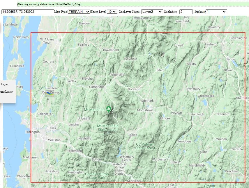
10.3.2 Typical layer configurations
| System | Layers (top to bottom) | Typical K (m/day) | Typical thickness (m) |
|---|---|---|---|
| Glacial-drift + bedrock | Surficial sand/gravel (aquifer) | 10 – 100 | 10 – 50 |
| Till (confining) | 10-4 – 10-2 | 2 – 20 | |
| Weathered bedrock (deep aquifer) | 0.1 – 5 | 20 – 100+ | |
| Coastal plain aquifer system | Surficial sand | 10 – 50 | 10 – 30 |
| Clay confining unit | 10-5 – 10-3 | 5 – 30 | |
| Confined sand aquifer | 10 – 100 | 30 – 100 | |
| Alluvial + bedrock | Alluvium (high-K) | 50 – 500 | 5 – 30 |
| Weathered bedrock zone | 0.1 – 10 | 5 – 30 | |
| Competent bedrock (deep aquifer or effectively no-flow) | 0.001 – 1 | variable |
Confining units are the heart of most multi-layer questions — they control how much water moves between aquifers. Three parameters govern their behavior:
- Vertical hydraulic conductivity (Kz) — typically 10-6 to 10-3 m/day for clay-rich units, 10-3 to 10-1 m/day for sandy confining layers.
- Thickness — directly controls the vertical conductance: the thinner the confining unit, the more leakage. Windows or breaches in the confining unit (zero-thickness zones) can completely compromise confinement.
- Specific storage — for transient problems, the confining unit stores water compressibly. This is how wells near a confining unit can see delayed responses.
10.4 Layer Elevations and Geometry
Layer elevations — the top and bottom of each conceptual layer — are what give the model its vertical structure. Getting them right takes real data about the subsurface, and the platform offers the same customization ladder for elevations that it does for K and recharge.
10.4.1 The customization ladder for layer elevations
For each layer's top and bottom, you climb the same rungs that Chapter 5 §5.2 established for any spatial attribute:
| Rung | Method | When to use |
|---|---|---|
| 1 | Platform default (DEM for top of layer 1, "DEM minus constant" for layer 1 bottom) | Unlayered base model — fine for first pass |
| 2 | User-specified constant | Simple layered system with approximately flat geologic contacts |
| 3 | Data Center raster — bedrock elevation, aquifer-top raster, aquifer-bottom raster | Most real-world work — authoritative spatially-variable layer surfaces |
| 4 | Uploaded raster — site-specific layer surfaces from local data | Detailed site investigations with better-than-Data-Center data |
| 5 | Scattered points with interpolation (IDW, Natural Neighbor, Kriging) | Borehole elevation picks — e.g., top-of-confining-unit from lithology logs |
| 6 | T-PROGS realization (Ch. 16) | Geostatistical characterization with multiple material categories |
10.4.2 Ensuring layers align
Adjacent conceptual layers must share a boundary surface: the bottom of layer 1 equals the top of layer 2, and so on. If they don't — if there's a gap or overlap between layer 1's bottom and layer 2's top — the solver either leaves an unresolved region (gap) or double-counts material (overlap), both of which produce garbage results.
In IGW-NET, the platform enforces this: when you set the bottom of layer 1 to a raster, the top of layer 2 is automatically set to the same raster. You only need to specify each internal boundary once.
When using scattered borehole points to define a confining-unit top, two boreholes may report slightly different elevations at nearby locations — not because the contact is really that variable, but because the picks were made by different geologists using different criteria. The interpolated surface smooths these out, but only partially. If layer geometry matters for your question, verify a few well locations by walking the interpolated surface against borehole logs; adjust picks if the interpolation is clearly fighting the data.
10.4.3 Pinchouts and unconformities
Real geologic contacts don't always stay neatly horizontal. Two common complications:
- Pinchouts — a confining unit that exists in one part of the domain but not another. Where the unit pinches out, the two aquifers above and below it are in direct hydraulic contact.
- Unconformities — layer contacts that are angled, cut by erosion, or truncated by younger deposits. The elevation of a layer's top is not a smooth function of horizontal position.
IGW-NET handles these by allowing zero-thickness regions: where the confining unit's thickness goes to zero, the solver effectively connects the aquifer above and below it directly. Zones (Ch. 6 §6.2) can be used to locally override layer attributes or force a layer to be absent in a specific area.
10.5 Inter-Layer Communication
Once you have multiple conceptual layers, the question of how water moves between them becomes central. This is governed by vertical hydraulic conductivity, confining-unit integrity, and (for transient problems) confining-layer storage.
10.5.1 The physics — vertical Darcy flow
Vertical flow between a cell in layer 1 and the corresponding cell in layer 2 follows the same Darcy's law that governs horizontal flow, but with vertical K replacing horizontal K:
qvertical = - Kz,effective × (hupper - hlower) / dvertical
Where:
Kz,effective— harmonic mean of the vertical K's of the two layers plus any intervening confining unithupper, hlower— computed heads in the two layersdvertical— vertical distance between layer centers
Two consequences:
- Vertical flow goes from higher to lower head, regardless of which layer is "upper." An artesian lower layer — with head higher than the upper layer's head — pushes water upward. This is exactly the physics behind artesian wells and upwelling through aquitard windows.
- A confining unit with very low Kz dominates the harmonic mean. Even thin aquitards can effectively decouple the layers if Kz is small enough.
10.5.2 Anisotropy — horizontal vs vertical K
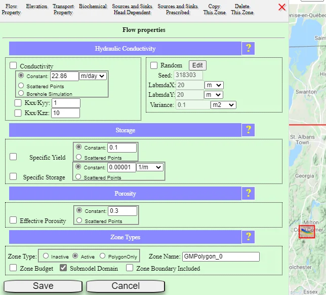
Real aquifers are almost never isotropic. Layered sedimentation, compaction, and preferred depositional fabric all tend to make horizontal K larger than vertical K — often by factors of 10 to 1000. This anisotropy is set in IGW-NET via the aquifer attributes dialog; in a typical layered aquifer you might specify Kh = 10 m/day with a Kh/Kz ratio of 100, meaning Kz = 0.1 m/day.
| Material | Typical Kh/Kz ratio |
|---|---|
| Well-sorted sand (high isotropy) | 2 – 10 |
| Typical alluvium with some bedding | 10 – 100 |
| Layered/interbedded sand and silt | 100 – 1000 |
| Fractured rock (depends on fracture orientation) | Highly variable; often >1000 for bedding-parallel fractures |
| Thin laminated clay and silt layers | 1000 – 10,000 |
Anisotropy is difficult to measure directly — you'd need vertical piezometers or dedicated vertical slug tests. So in practice, anisotropy is often a calibration parameter — you assume a plausible ratio (say, Kh/Kz = 100), run the model, compare to observations, and adjust the ratio if the model doesn't match the data. Chapter 17 covers how to do this systematically with UCODE.
10.5.3 Confining-unit storage (for transient problems)
In transient modeling, confining units don't just restrict vertical flow — they also store water compressibly. This matters because:
- When a stress is applied (e.g., pumping in a deep aquifer), the initial response is rapid drawdown drawing water from the aquifer itself. As time progresses, water begins to leak from the confining unit, slowing the drawdown but never fully stopping it until a new steady state is reached.
- The specific storage of the confining unit controls this delayed-leakage behavior. Clay units can have Ss of 10-4 to 10-3 m-1 — much higher than aquifer Ss (10-6 to 10-5).
- For aquifer tests in systems with significant confining-unit storage, the "type curve" shape reflects the combined aquifer-plus-confining-unit response, which is why Hantush-type semi-log analyses are needed rather than simple Theis.
10.6 Reading Multi-Layer Results
In a 2D model, you look at one head contour map. In a multi-layer model, you have multiple head fields — one per layer — plus vertical flow components between them. Interpretation takes practice.
10.6.1 Plan view per layer
The plan view in IGW-NET shows one layer at a time. A selector lets you switch between layers to see their independent head contours and flow vectors. What to look for:
- Different flow patterns between layers. The upper aquifer often responds strongly to topography — contours following rivers and ridges. A deeper confined aquifer may have a much smoother, regional gradient.
- Layer-specific features. A pumping well in layer 2 will show a cone of depression in layer 2 — but potentially little response in layer 1 if the confining unit is effective.
- Vertical communication zones. Look for plan-view locations where upper-layer and lower-layer heads differ most, or where they are nearly equal. Equal heads usually mean direct communication (confining unit absent or breached); strong head differences mean effective confinement.
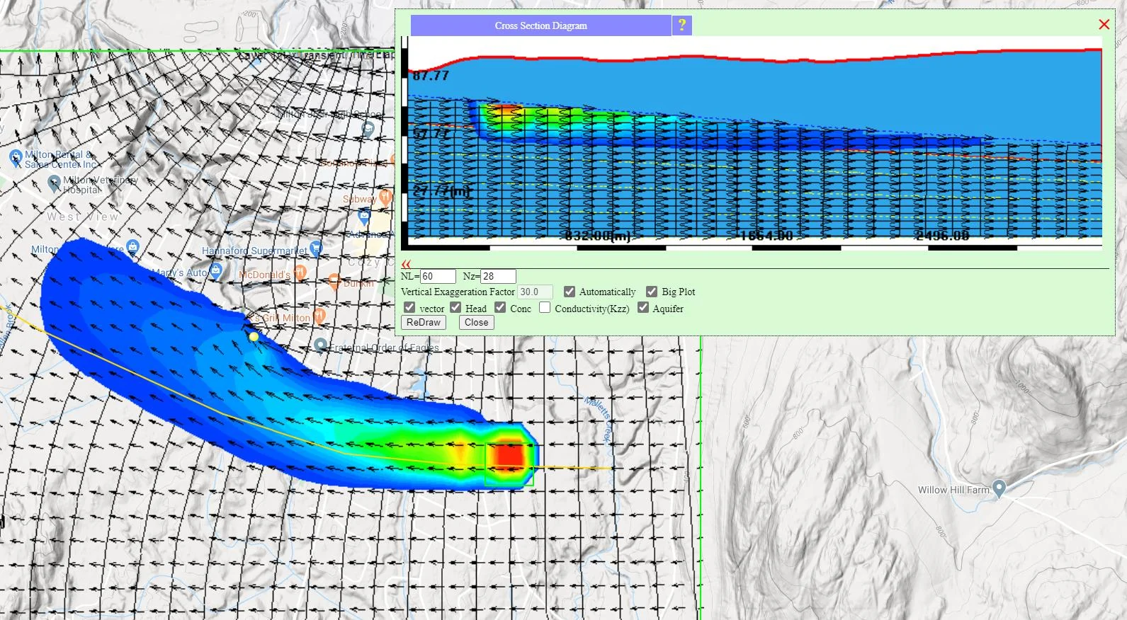
10.6.2 Cross-sections — the real reveal
Multi-layer results become interpretable when you draw cross-sections. Chapter 8 §8.3 introduced cross-sections; for multi-layer models, they become essential.
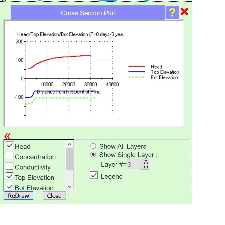
In a cross-section, you see:
- The physical geometry — layer thicknesses, pinchouts, undulating contacts — as drawn by the interpolated elevation surfaces.
- The hydraulic geometry — where heads are, where the water table is, the vertical flow pathways.
- The density of streamlines or velocity vectors through each layer, showing which layer is doing the work of moving water laterally.
- The plume or particle trajectories in transport/particle simulations, including vertical migration into or across confining units.
10.6.3 Water balance by layer
The water balance tool (Ch. 8 §8.4) reports per-layer inflows and outflows in multi-layer models. Key categories unique to multi-layer systems:
- Inter-layer flux — water moving between layers. Positive upward, negative downward (or vice versa, per platform convention). This is the total leakage through confining units.
- Storage by layer — how much water each layer is gaining or losing from its own storage (transient only). Confining-unit storage contributions show up separately.
Understanding the inter-layer flux is often the whole point of a multi-layer simulation. If your question is "how much contamination reaches the deep aquifer," the inter-layer downward flux at the relevant horizontal location is the quantitative answer.
Most horizontal questions can be answered in 2D. Most vertical questions cannot. "Does water move from aquifer A to aquifer B, and if so, how much?" — inherently vertical, needs multi-layer. "How quickly does a plume reach the deeper supply well?" — inherently vertical, needs multi-layer. When the decision-critical quantity is a vertical flux or a vertically-resolved concentration, 2D cannot answer it. That's when the extra complexity of multi-layer earns its keep.
To go deeper
- Chapter 12 — Contaminant Transport — next chapter. Transport in multi-layer systems is where vertical migration, breakthrough at deep receptors, and inter-layer leakage risk become central.
- Chapter 16 — T-PROGS 3D Geology — the geostatistical path to full 3D heterogeneity, beyond explicit layering.
- Chapter 17 — Calibration — calibrating multi-layer models, including anisotropy and inter-layer leakance as parameters.
- Ch. 7 §7.4 — Sublayers — the companion concept to conceptual layering.
- Quick Tutorial 10: Aquifer Layers — hands-on walkthrough of building a multi-layer model.
- Platform Concept: Layer Communication — the details of harmonic-mean K and vertical conductance.