The quick read — 90 seconds
- T-PROGS produces realistic 3D heterogeneous K fields from borehole data. Between "single K for the whole aquifer" (too simple) and "fully-detailed stratigraphic model" (too much) there's a sweet spot: geostatistically-simulated lithology that honors the boreholes you have and fills in the rest with statistically-consistent patterns.
- T-PROGS treats materials as categorical, not continuous. Each point in the aquifer belongs to a discrete material (sand, silt, clay, till) — not a smoothed K value. Transitions between materials are sharp, matching real geology.
- Contrast with alternatives. Kriging/IDW/Natural-Neighbor interpolate continuous K smoothly between wells — produces mathematical surfaces. Random fields simulate statistically-homogeneous heterogeneity — no honoring of observed stratigraphy. T-PROGS produces layered, observation-honoring 3D fields.
- Four classes: AQ / MAQ / PCM / CM. Aquifer (coarse sand/gravel, high K), Marginal Aquifer (fine/silty sand, moderate K), Partial Confining Material (silt/till, low K), Confining Material (clay/dense till, very low K). T-PROGS provides the spatial distribution; the modeler provides one K value per class — four scalar parameters characterizing the entire 3D heterogeneous K field.
- Regional zonation when geology varies across the domain. If different parts of the domain have meaningfully different geologic settings (glaciated vs. unglaciated, different physiographic provinces, different depositional environments), divide into spatial regimes — each zone with its own set of four class K values. Parameter count scales linearly: N zones × 4 = 4N parameters. Zonation complexity is bounded by how much calibration data you have, not by geologic ambition. See §17.5.
- Setup in IGW-NET: DM Zone → Flow Properties → Conductivity → Borehole Simulation → Import .tp file → Material K table. Five-step workflow; four class K values go in the table (Barron Lake: 53, 5, 0.01, 0.001 ft/day for AQ, MAQ, PCM, CM respectively).
- Regional data coverage: approximately 10 U.S. states, plus all Canadian provinces. Water-well lithology databases are integrated into DataNET for automated borehole ingestion — T-PROGS runs server-side, .tp file delivered to IGW-NET. Wellogic (Michigan) is one instance; other covered states and all Canadian provinces have equivalent integrations. Outside the covered regions, users supply their own borehole data.
- Use T-PROGS when stratigraphic control matters (layered aquifers, confining units, transport with preferential flow paths), borehole data is available or auto-integrated, glacial terrain with discrete lithology.
- Skip T-PROGS when simple regional questions where bulk K suffices, no borehole data and no automated coverage, steady-state models where regional head pattern is the output.
- Works best with vertical layering (Ch. 10) — 3–5 layers typical for capturing stratigraphy in depth. Single-layer T-PROGS works but loses much of the vertical-heterogeneity value.
Chapter 17 — T-PROGS 3D Geology
17.1 Why T-PROGS Exists — Between Single-K and Full Stratigraphy
Every groundwater model has to decide how to represent the aquifer's conductivity. The choices span a spectrum from very simple to very detailed; T-PROGS occupies a specific, useful middle ground that most modeling benefits from when the data supports it.
17.1.1 The spectrum of K representations
| Representation | What it is | When it works | When it fails |
|---|---|---|---|
| Single bulk K | One constant K value across the entire aquifer (or per zone) | Regional models with well-behaved homogeneous aquifers; demonstrations; first-pass calibration | When stratigraphic heterogeneity actually matters for the question |
| Scattered-point interpolation | K values at wells interpolated smoothly between them via IDW, Natural Neighbor, or Kriging | When K varies gradually and wells are reasonably dense | Real geology is layered, not smoothly-varying; smooths out sharp contacts that matter hydraulically |
| Random fields | Statistically-generated spatially-correlated K field with specified variance and correlation length | When no borehole data exists and bulk heterogeneity magnitudes need representation | Doesn't honor observed stratigraphy; each realization is unrelated to the actual geology |
| T-PROGS | Geostatistical simulation of categorical materials from borehole data | Borehole data available; stratigraphy matters; realistic-looking heterogeneity needed | No boreholes; very large regional models where bulk K suffices; steady-state only |
| Full stratigraphic model | Hand-constructed geological surfaces defining each lithologic unit | Site-scale detailed studies where every unit is characterized | Setup cost enormous; overkill for regional modeling |
T-PROGS sits between scattered-point interpolation and full stratigraphic modeling — more realistic than smoothed K surfaces but far cheaper than hand-constructing every geological unit. It uses the borehole data you have to inform a statistical model of stratigraphy, which then generates K fields consistent with the observations.
17.1.2 What "realistic" means here
The central claim of T-PROGS: the K fields it produces look like geology. Concretely:
- Discrete lithologic units. You see distinct sand layers, clay lenses, till beds — not smooth color gradients. This matches what geologists see in cross-sections and well logs.
- Sharp contacts between units. A sand layer meets a clay bed along a distinct contact surface, not a gradual transition. K changes by orders of magnitude across that contact.
- Realistic geometry. Layers have appropriate thickness, lateral continuity, and proportions matching what borehole observations suggest. Sand lenses are lens-shaped, not spherical blobs.
- Stratigraphic ordering. Younger deposits sit on older, with transitions following geological reasonable patterns (a sand unit doesn't typically sit directly on bedrock without an intervening till in glacial terrain, for example).
- Borehole honoring. At every borehole location, the simulated lithology matches the observed record exactly — the data is not smoothed or averaged.
These are qualitatively different fields from what continuous interpolation produces. A sandy aquifer with a clay lens will show, in T-PROGS output, an actual clay lens with sharp edges; in kriged output, the same aquifer shows a K minimum that smoothly decreases and increases through the clay area. The hydraulic behavior differs: the T-PROGS clay lens diverts flow; the kriged minimum only partially impedes it.
17.1.3 The four-class typology — AQ, MAQ, PCM, CM
T-PROGS produces a categorical field — every cell belongs to a discrete material class. IGW-NET uses a standard four-class typology grounded in hydrogeologic function rather than in lithologic description alone:
| Class | Full name | What it represents | Typical K range |
|---|---|---|---|
| AQ | Aquifer | Coarse sand, gravel, clean outwash — the productive water-bearing units that transmit groundwater freely | ~10 to 100+ ft/day |
| MAQ | Marginal Aquifer | Fine sand, silty sand, transitional materials — transmits water but with meaningfully reduced capacity | ~1 to 10 ft/day |
| PCM | Partial Confining Material | Silt, sandy till, mixed fine materials — substantially impedes vertical flow but doesn't fully confine | ~0.001 to 0.1 ft/day |
| CM | Confining Material | Clay, dense till, impermeable bedrock — functionally an aquitard at groundwater modeling time scales | < 0.001 ft/day |
The typology is hydrogeologic, not lithologic. Drillers describe lithology in many ways — "coarse gravelly sand", "silty clay with stones", "weathered shale" — but what matters for groundwater modeling is how the material transmits water. AQ/MAQ/PCM/CM groups the thousands of possible lithologic descriptions into four classes organized by hydraulic function. "Gravelly sand" and "coarse outwash" are both AQ because they both transmit water freely; "silty clay" and "glacial till with high clay fraction" are both CM because they both effectively block flow.
Four classes strike a balance between two competing pressures:
- Simple enough to calibrate. T-PROGS provides the spatial distribution of classes (from the borehole data); the modeler provides a K value for each of the four classes. That's four scalar parameters characterizing the entire 3D heterogeneous K field — orders of magnitude fewer parameters than hand-specifying K everywhere, yet capturing the essential heterogeneity structure. For calibration (Ch. 18), four K values per model is tractable; four hundred wouldn't be.
- Rich enough to capture real aquifer behavior. The full K spectrum in most sedimentary aquifers spans about six orders of magnitude (coarse gravel at 1000 ft/day to dense clay at 0.0001 ft/day). Four classes give you roughly one class per two orders of magnitude of K — enough resolution to distinguish aquifers from marginal aquifers from aquitards, which is the functional distinction that controls groundwater flow.
The result: T-PROGS gives you a 3D field of tens of thousands to millions of cells, each with a specific K value, but that entire field is characterized by just four numbers (the four class K values) plus the spatial pattern (from the .tp file). Four parameters; full 3D heterogeneity. This is what makes T-PROGS practical.
Throughout this chapter, material categories are referred to both by their class labels (AQ, MAQ, PCM, CM) and by the material numbers (1, 2, 3, 4) they appear as in the Borehole Simulation Options dialog. Material 1 = AQ, material 2 = MAQ, material 3 = PCM, material 4 = CM is the standard mapping.
17.2 Transition Probability Geostatistics — The Method
This section gives an intuition for what T-PROGS is actually doing under the hood. Full geostatistical theory is beyond this manual's scope, but understanding the core idea helps you use T-PROGS well and recognize when its assumptions apply.
17.2.1 The core idea — transitions between materials
Rather than modeling K as a continuous random variable, T-PROGS models the probability of transitioning between material categories as you move through space. Given you're currently in "sand" at some location, what's the probability the next point (in some direction, at some distance) is also "sand" versus "clay" versus "till"?
This probability structure — the transition probability — is estimated from the borehole data:
- Proportions — how much of the observed lithology is each material (e.g., "30% sand, 20% silt, 40% till, 10% dense till")
- Mean lens thickness — in each direction (vertical, horizontal), typical thickness of each material (e.g., "sand lenses average 3 m thick vertically, 50 m laterally; till beds average 8 m thick vertically, 500 m laterally")
- Juxtaposition tendencies — which materials tend to occur next to each other (sand often adjacent to silt; clay rarely directly adjacent to dense till without intervening layers)
From these statistics, T-PROGS simulates realizations — specific 3D arrangements of materials that are statistically consistent with the observed structure. Each realization honors the boreholes exactly (observed material at observed depth, at the observed location) and fills in between with materials distributed per the transition probability model.
17.2.2 Why categorical treatment matters
The categorical framing is the key distinguishing feature of T-PROGS. Kriging and similar continuous-interpolation methods assume K is a smooth function of space with some uncertainty. Transition probability methods assume the material type is a discrete choice at each point, with spatial structure governing how those choices cluster into layers and lenses.
This matters because:
- Real lithology is discrete — you don't have "62% sand" at a point; you have sand or you have clay. The categorical model matches the data-generating process.
- K contrasts are preserved — a 5000× K contrast between sand and clay shows up as a 5000× contrast in the simulated field. Continuous interpolation would smooth this contrast and lose most of the hydraulic effect.
- Flow behavior is different — preferential flow along high-K channels, flow focusing at stratigraphic windows, and stagnant zones in low-K pockets all require the sharp contrasts that categorical simulation preserves.
For readers familiar with geostatistics: T-PROGS is conceptually related to indicator kriging (both handle categorical variables) but uses transition probabilities directly rather than variograms of indicator variables. The practical advantage is that transition probabilities are more interpretable — "mean sand thickness = 3 m" is a direct geological statement, while an indicator variogram is an indirect statistical quantity. Both produce similar results when parameterized consistently; T-PROGS' formulation is more convenient for geologists to parameterize from standard lithologic descriptions.
17.2.3 What T-PROGS doesn't do
Important limits to understand:
- T-PROGS simulates structure, not properties within each material. Each material has one Kxx value (and optionally Kxx/Kyy, Kxx/Kzz ratios); within the material, K is constant. For finer-grained heterogeneity within a single lithologic category, you'd overlay random fields or use a more refined material classification.
- T-PROGS is statistical, not deterministic. Different runs produce different realizations — all consistent with the borehole data and the transition probability statistics, but differing in where specific lenses are between wells. For critical applications, multiple realizations can be run and compared (stochastic simulation, Ch. 19).
- T-PROGS needs data. Without boreholes, there's nothing to estimate transition probabilities from. For regions without borehole data, T-PROGS isn't the right tool.
- T-PROGS doesn't model specific geological processes. Glacial outwash, fluvial channels, delta progradation, lacustrine sequences — these have specific depositional signatures that a process-based geological model would capture. T-PROGS captures their statistical end-product but not the processes.
17.3 Setup — The Borehole Simulation Workflow
In IGW-NET, T-PROGS is accessed through the Zone Flow Properties → Conductivity → Borehole Simulation option. This section walks through the five-step workflow.
17.3.1 The workflow
Create a DM Zone covering the entire model domain
Zones → Zone = DM (or equivalent zone-type selection). The DM (Domain Material) Zone is the zone that T-PROGS will populate with heterogeneous K. For most models this zone covers the whole aquifer; you can have sub-zones inside it for specific features (contaminant source areas, excluded regions) that override with different K.
Open Zone Attributes → Flow Properties → Conductivity
In the Flow Properties tab of the Zone Attributes dialog, check Conductivity to enable K configuration for this zone. Under Conductivity, the sub-option radio buttons let you choose: Constant, Scattered Points (IDW/Natural-Neighbor/Kriging), Random Fields, or Borehole Simulation. Select Borehole Simulation.
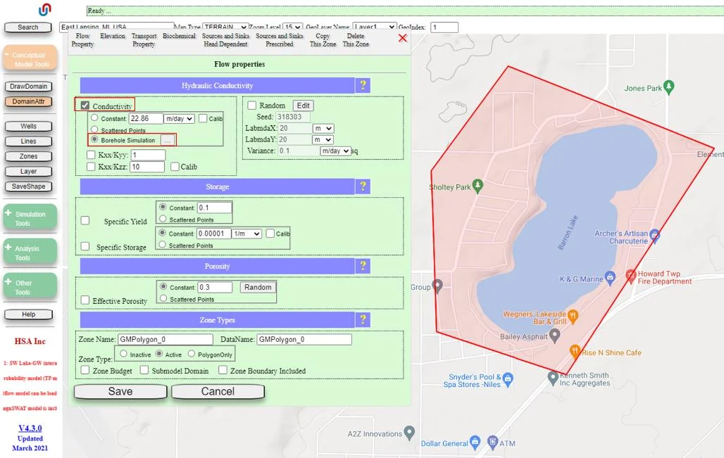
Open Borehole Simulation Options
Click the '...' options button next to Borehole Simulation. The Borehole Simulation Options dialog opens — this is the main T-PROGS configuration panel.
Import the .tp file
Check Import and upload your .tp file (BarronLakeTP.tp in the Barron Lake case). The .tp file is the T-PROGS output — the 3D categorical material field. For automated-coverage regions, the Data Center delivers this file pre-computed; for other regions, you produce it from an upstream T-PROGS workflow.
Configure the Material table
The Material table has one row per material type with columns for Kxx, Kxx/Kyy, Kxx/Kzz, porosity, Sy, and Ss. For each material, fill in the K value — the central parameter — plus anisotropy ratios and storage parameters. These convert the categorical material field (integer material IDs 1, 2, 3, ...) into the actual K values and properties used by the simulation.
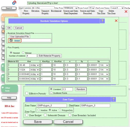
BarronLakeTP.tp imported and the Material table showing 4 materials. Kxx values are 53, 5, 0.01, and 0.001 ft/day for Material 1 through Material 4 respectively. Default Kxx/Kyy and Kxx/Kzz ratios (typically 1 and 10 respectively for glacial deposits) work well for most starting points.17.3.2 Material K values — the central parameter
The most important input is the Kxx (horizontal conductivity) per material. Using the four-class typology introduced in §17.1.3, typical K ranges per class:
| Class | Typical lithologies | Kxx (ft/day) | Kxx (m/day) | Barron Lake value |
|---|---|---|---|---|
| AQ (Aquifer) | Clean sand, outwash, gravel; coarse sand-dominated units | ~10 to 100+ | ~3 to 30+ | 53 |
| MAQ (Marginal Aquifer) | Fine sand, silty sand, transitional deposits | ~1 to 10 | ~0.3 to 3 | 5 |
| PCM (Partial Confining Material) | Silt, silty till, loamy till, mixed fine materials | ~0.001 to 0.1 | ~0.0003 to 0.03 | 0.01 |
| CM (Confining Material) | Clay, dense till, impermeable bedrock | < 0.001 | < 0.0003 | 0.001 |
These are typical starting values; calibration (Ch. 18) often refines them based on observed heads and fluxes. The important thing is to get the orders of magnitude right — AQ should be ~10,000× more permeable than CM, not 10× — because the hydraulic behavior depends on the K contrast between productive units and confining layers. The Barron Lake values in the rightmost column fall squarely within the typical ranges; they represent specific tunings for that site's glacial stratigraphy (§17.4).
The practical power of the 4-class typology: four scalar K values, together with the spatial class distribution from T-PROGS, fully characterize the aquifer's 3D K field. You're not adjusting thousands of parameters — you're adjusting four. For calibration, for sensitivity analysis, for uncertainty quantification, four parameters is tractable. This is what makes T-PROGS practical for routine modeling rather than a research-only technique.
17.3.3 Anisotropy ratios
Kxx/Kyy and Kxx/Kzz ratios capture directional variation in K within each material:
- Kxx/Kyy (horizontal anisotropy) — typically 1 (isotropic) for most glacial deposits. Can be elevated for alluvial fan deposits with preferred flow direction, but that's unusual in most groundwater contexts.
- Kxx/Kzz (vertical anisotropy) — typically 10 for glacial deposits (horizontal K 10× vertical K, reflecting layered deposition). Can be higher (50, 100) for highly-laminated sediments; can be 1 for massive rock or isotropic materials.
The IGW-NET defaults (Kxx/Kyy = 1, Kxx/Kzz = 10) work well for most glacial-terrain applications. Site-specific calibration may adjust them.
17.4 The Barron Lake 4-Material Example
Barron Lake's T-PROGS configuration is an instructive example of how glacial stratigraphy maps onto the 4-material T-PROGS framework. This section unpacks the specific choices.
17.4.1 The 4 materials
The Barron Lake model uses the standard 4-class T-PROGS typology (§17.1.3), with K values tuned to the observed glacial stratigraphy in southwest Michigan:
| Class | Material (in .tp) | Lithology at Barron Lake | Kxx (ft/day) | Role in the aquifer system |
|---|---|---|---|---|
| AQ | Material 1 | Outwash sand and gravel | 53 | The primary aquifer; where wells pump; strongly transmits water |
| MAQ | Material 2 | Fine sand / silty sand | 5 | Marginal aquifer; transitional between outwash and confining layers |
| PCM | Material 3 | Till (sandy, loamy) | 0.01 | Partial confining material; local aquitards that slow vertical flow |
| CM | Material 4 | Dense till / clay | 0.001 | Confining material; effective aquitard at the base |
The K values span 5 orders of magnitude (from 53 to 0.001 ft/day = 53,000× contrast) — capturing the full range of permeabilities in the glacial deposits. This is the hydraulically-realistic range; a single bulk K would average all four into something like 1 ft/day, missing both the productive aquifer behavior and the confining-layer effects. Note that the class values for Barron Lake (53, 5, 0.01, 0.001 ft/day) fall squarely within the typical class ranges given in §17.1.3 — they are project-specific tunings within the standard typology, not free-parameter choices. The four K values together characterize the entire 3D heterogeneous K field that T-PROGS produces from the borehole data.
17.4.2 How the stratigraphy plays out in 3D
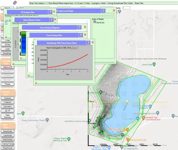
17.4.3 Why this structure matters for the Barron Lake model
The stratigraphic heterogeneity is not cosmetic — it affects the model's answers:
- Lake-aquifer coupling strength depends on the K of the material directly beneath the lake. If the lake sits on outwash (Material 1), exchange is strong; if it sits on till (Material 3 or 4), exchange is weak. T-PROGS tells you which.
- Well yield patterns depend on which stratigraphic units the well intersects. Wells screened in outwash yield well; wells in silty sand yield modestly; wells in till yield poorly. The 11 private wells in the Barron Lake study have different productivity based on their screened units.
- Contaminant transport preferential paths follow high-K units. A spill at the lake edge migrates rapidly through outwash lenses and slowly through surrounding till — pattern invisible in single-K models.
- Regional flow organization — the mainstem regional flow follows high-K units between lower-K confining layers, producing the layered flow patterns observable in detailed head measurements.
17.5 Regional Zonation — When One Set of 4 Parameters Isn't Enough
The Barron Lake single-zone configuration is the baseline T-PROGS setup: four K values for the whole domain, characterizing the complete 3D heterogeneous K field. For larger or geologically more complex models, a single set of four values may not capture spatial variation in the underlying geology. This section covers when and how to escalate from one-zone to multi-zone T-PROGS.
17.5.1 Why regional zonation is needed
The four-class typology (§17.1.3) groups materials by hydraulic function — AQ is coarse-grained productive units, CM is fine-grained aquitards. But what counts as an AQ in one region may be hydraulically different from AQ in another region. Two examples:
- Glacial outwash AQ vs. fluvial fan AQ. A glacial outwash aquifer (clean sorted sand, modest K around 50 ft/day) and a fluvial fan aquifer (cobbles and coarse gravel with high K around 500 ft/day) are both "AQ" — both are the most productive unit in their region — but their K differs by an order of magnitude. Using a single AQ parameter for both misrepresents one or the other.
- Glaciated vs. unglaciated terrain. In glaciated terrain, CM is typically dense till (K around 0.001 ft/day). In unglaciated sedimentary terrain, CM might be shale or claystone (K closer to 0.0001 ft/day, ten times lower). A model crossing the glacial boundary would need different CM values on each side.
When the domain spans meaningfully different geologic settings — physiographic provinces, glaciated boundaries, depositional environments, bedrock geology changes — one set of four parameters can't capture the full variation. The solution: divide the domain into spatial regimes or zones, each with its own set of four K values.
17.5.2 How regional zonation works
Each spatial regime is defined as a zone (using IGW-NET's standard zone infrastructure, same as for submodels in Ch. 13). Within each zone, T-PROGS produces its own 3D categorical material distribution, and the four class K values (AQ, MAQ, PCM, CM) are specified per zone. The total parameter count scales linearly with the number of zones: N zones × 4 class K values = 4N parameters.
| Zone count | Parameters | Calibration target count needed | Typical use |
|---|---|---|---|
| 1 zone (baseline) | 4 parameters | ~10+ observations | Single geologic province (like Barron Lake in a uniform glacial setting) |
| 2 zones | 8 parameters | ~20+ observations distributed across both | Domain spanning a boundary (glaciated/unglaciated, two provinces) |
| 3–4 zones | 12–16 parameters | ~30–40+ observations distributed across zones | Regional model covering multiple physiographic provinces |
| 5+ zones | 20+ parameters | ~50+ observations | Large multi-basin models where careful zonation matters |
Each additional zone adds four parameters and requires the calibration data to constrain them. The zone count shouldn't exceed what the observational data can constrain — more zones without supporting data produces an underdetermined calibration where multiple K-field configurations fit the observations equally well (non-uniqueness).
17.5.3 How to decide where zone boundaries go
Zone boundaries should follow real geologic contrasts, not arbitrary convenience. Useful guides:
- Physiographic maps. National or regional physiographic province maps (USGS for the US, provincial surveys for Canada) show where geologic settings change. These boundaries are usually appropriate T-PROGS zone boundaries.
- Surficial geology maps. Where the surficial geology changes — glacial to interglacial, moraine to outwash, alluvium to bedrock — the near-surface aquifer materials likely change, and zonation is warranted.
- Known aquifer-system boundaries. Published regional groundwater studies often delineate distinct aquifer systems with different properties. Use those boundaries.
- Observed head patterns. If your initial single-zone model calibration shows systematic regional biases in residuals (all wells in the north biased low, all wells in the south biased high), the residual pattern itself suggests where zonation might help.
The temptation: "my calibration shows bias between east and west; let me draw a zone boundary that separates them." This is overfitting dressed up as geologic reasoning. Zone boundaries should reflect prior geologic knowledge, not post-hoc residual patterns. If residuals suggest zonation, check whether geologic maps actually show a boundary in that location; if yes, zonation is legitimate. If no, the residual pattern probably reflects something else (unmodeled recharge variation, local heterogeneity, observation errors) and adding a zone boundary just masks the real issue.
The cleanest practice: define zones from geology before calibration; let the calibration refine the four K values per zone; evaluate residuals for remaining systematic patterns.
17.5.4 Escalation path — when to add zones
The practical workflow: start simple, add zones only when evidence demands.
Begin with one zone (the whole domain)
4 parameters (AQ, MAQ, PCM, CM). Run the T-PROGS simulation; calibrate the four K values (Ch. 18); evaluate residuals against observed heads and other targets.
Check residuals for systematic regional patterns
Are residuals scattered randomly around zero, or do they cluster spatially (one region consistently biased high, another consistently biased low)? Random scatter suggests the single-zone model is capturing the main variation. Systematic regional bias suggests regional zonation might help.
Check geologic maps for matching boundaries
If residual patterns align with physiographic or geologic province boundaries, zonation along those boundaries is justified. If not, investigate other causes (recharge variation, boundary conditions, observation quality) before adding zones.
Add zones one at a time
Split the domain into two zones at the most obvious geologic contrast first. Re-run and re-calibrate. See if residuals improve. If more zones are needed, add them incrementally with a geologic rationale for each.
Stop when residuals are acceptable or data limits are reached
If further zones don't improve the calibration meaningfully, or if you don't have enough observations to constrain the additional parameters, stop. Parameter count should always be matched to observational constraint.
17.5.5 Connection to calibration (Ch. 18)
Regional zonation directly affects calibration strategy. With 4 parameters per zone, the calibration is well-posed as long as you have enough observations per zone. Typical rule of thumb: at least 5–10 meaningful observations per 4 calibrated parameters, distributed so each parameter is independently constrained. Chapter 18 covers calibration mechanics, UCODE parameter estimation, and residual interpretation in detail — zonation is one of the first design decisions that shapes the calibration problem.
Zonation complexity is bounded by calibration data availability, not by geologic ambition. A domain spanning three physiographic provinces but with observations only in one province should still be modeled as one zone — the other two provinces' four parameters would be unconstrained. As more observations become available in the currently-data-poor regions, zonation can be added. The model complexity grows with the data; never ahead of it.
17.6 Regional Data Coverage — Water-Well Lithology Integration
T-PROGS needs borehole data. What makes it practical for day-to-day modeling is automated access to water-well lithology databases for a meaningful portion of North America.
17.6.1 The covered regions
DataNET integrates water-well lithology databases for:
- Approximately 10 U.S. states — state-specific water-well record databases (Michigan's Wellogic is the prototype; other covered states have similar state-run databases)
- All Canadian provinces — each province maintains a water-well database; all are integrated
Within the covered regions, the end-to-end T-PROGS workflow is automated through the Data Center:
You select a model domain anywhere in the covered region
Zoom in, draw the domain, confirm boundaries.
Request borehole data for the domain
Through the Data Center borehole integration option. DataNET identifies all water-well records within the domain, pulls their lithology logs, and formats them for T-PROGS ingestion.
T-PROGS runs server-side on MAGNET4WATER infrastructure
Estimates transition probabilities from the borehole data; generates a 3D categorical material realization; writes the .tp file.
The .tp file is delivered back to IGW-NET
Ready to be imported via the Borehole Simulation Options dialog (§17.3.1 step 4).
You configure material K values and simulate
The material table (§17.3.1 step 5) converts material IDs into K values; the aquifer is ready.
For regions outside the covered coverage, the methodology is identical but the data-acquisition path requires user involvement: users supply borehole data from whatever local source is available (USGS NWIS for US federal data, national geological survey databases for other countries, site-specific drilling records for local projects) in the T-PROGS input format.
17.6.2 Wellogic and its equivalents
Michigan's Wellogic is the most widely-referenced example of a state water-well database integrated with MAGNET4WATER. It contains lithologic logs from tens of thousands of wells drilled across Michigan over decades of well construction, documented by drillers as a regulatory requirement. The depth of coverage — one well every few hundred meters in developed areas — provides excellent T-PROGS input for most Michigan groundwater modeling.
Other covered states have equivalent state-run databases with comparable coverage (the exact name and administrative context varies by state). The DataNET integration abstracts these differences: regardless of which state you're in, the workflow is the same — request borehole data, receive the .tp file.
Canadian provincial databases operate similarly, maintained by each province's water-resources or environment ministry, with coverage determined by provincial well-drilling records.
The fastest way to confirm T-PROGS coverage for a specific location: in IGW-NET, draw a small domain and try the Data Center borehole request. If data is returned, the region is covered. If not, you'll need to supply borehole data manually. The coverage can change over time as new integrations are added; the Data Center is the source of truth for current availability.
17.7 When to Use T-PROGS
T-PROGS adds configuration complexity and interpretation overhead. This final section helps you decide whether that cost is worth paying for your specific modeling question.
17.7.1 Strong signals for T-PROGS
Use T-PROGS when any of these apply:
- Stratigraphic control is known to matter. You have prior knowledge — from consulting reports, regional hydrogeologic assessments, or past calibration experience — that the aquifer is meaningfully layered and that heterogeneity drives behavior.
- Transport modeling (Ch. 12). Contaminant transport is especially sensitive to preferential flow paths. T-PROGS reveals the high-K lenses that route plumes; smoothed K fields miss them.
- Wellhead protection in complex geology. Delineating capture zones in layered aquifers with confining units requires realistic vertical structure.
- Coupled-lake modeling (Ch. 15) in glacial terrain. The K directly beneath the lake controls the coupling strength; T-PROGS gives you a defensible value.
- Client or regulatory expectations for realistic-looking 3D geology. Cross-sections and 3D visualizations are much more convincing with T-PROGS heterogeneity than with smoothed fields.
- Automated data coverage. Your domain is in the 10 covered U.S. states or any Canadian province — the setup cost is minimal, so the threshold for using T-PROGS drops.
17.7.2 Signals to skip T-PROGS
Skip T-PROGS when:
- Bulk K is sufficient for the question. Regional flow pattern; long-term water balance; first-pass scoping studies.
- No borehole data available. Outside covered regions without user-supplied data, T-PROGS has nothing to work with. Use scattered-point interpolation of whatever wells you do have, or a random-fields approach.
- Steady-state models where head pattern is the primary output. Calibrating a bulk K often matches observed heads as well as calibrated T-PROGS K values would, at a fraction of the setup cost.
- Very large regional models where computational cost of 3D heterogeneous K is prohibitive.
- Homogeneous aquifers. Some aquifers really are nearly uniform — thick sandstone formations, massive carbonate platforms. T-PROGS on these is overkill and the result is indistinguishable from bulk K.
17.7.3 The escalation path
The recommended workflow for most new models: start with bulk K (or scattered-point interpolation if wells are dense enough). Calibrate the model; check whether the simple K representation matches observations. If calibration is poor in ways suggesting stratigraphic control — e.g., head patterns that don't respond to bulk-K changes, wells with anomalously different behavior than neighbors, transport plumes with unrealistic shapes — escalate to T-PROGS. This escalation is straightforward if your region is covered (just request borehole data and re-run); more involved if you need to supply your own data.
Don't escalate to T-PROGS as a first move unless you have specific stratigraphic-control reasons upfront. The setup cost is real, and many models don't need the complexity it adds.
To go deeper
- Chapter 5 — Aquifer Attributes — the foundation; bulk K and zone-based K options that T-PROGS extends with stratigraphic detail.
- Chapter 10 — Vertical Layering — essential companion; T-PROGS produces 3D fields that need vertical layers to resolve.
- Chapter 12 — Transport — where T-PROGS' stratigraphic detail most affects outcomes; preferential flow paths in high-K lenses.
- Chapter 15 — Coupled Lake-Aquifer Modeling — coupled-lake K beneath the lake; often paired with T-PROGS for realistic coupling.
- Chapter 18 — Calibration with UCODE — calibrating material K values using observed heads and fluxes.
- Chapter 19 — Stochastic & Monte Carlo — multiple T-PROGS realizations as the basis for uncertainty quantification.
- Case Study: Barron Lake Coupled Model — the full end-to-end example with T-PROGS configuration, material K values, and cross-sections.