The quick read — 90 seconds
- The Watershed Solver is IGW-NET's in-platform subsystem for watershed processes. When enabled, it computes overland flow, infiltration, runoff, and channel routing alongside the aquifer solve. When not enabled, recharge is treated as a pre-computed input (uniform value or raster) and surface-routed water is not modeled.
- Enable it when coupled lakes (Ch. 15) need runoff Ins; when you want recharge to respond to rainfall patterns dynamically; when channel or stream routing matters; when seasonal rainfall variability matters. Don't enable it when pre-computed recharge is adequate, the model is steady-state, or you have no SW features that depend on surface-routed water.
- Configured through three tabs in the Surface Water Overland Flow Options dialog. Land Use and Cover (with Manning's coefficient), Climate (rainfall and evaporation), Soil Type (infiltration parameters). All three typically drawn from the Data Center as starting defaults.
- Manning's coefficient is stored everywhere but active only when the Watershed Solver is enabled. Users often configure Manning's n expecting it to matter and see no simulation response — because the Watershed Solver is off. If you see Manning's n in attribute dialogs but your simulation doesn't respond to changes, that's why.
- Seasonal rainfall patterns — the Watershed Solver supports four seasons (Summer, Fall, Winter, Spring) each with configurable hours-per-day and date ranges, so rainfall variability can be captured without requiring full climate time series.
- Infiltration-as-recharge is the coupling option that takes the Watershed Solver's infiltration calculation and feeds it directly as GW recharge — per cell, per time step, responding to actual rainfall events and landscape properties.
- Channel and stream routing model surface water flowing through the stream network, enabling more physically realistic stream-aquifer coupling than fixed-stage Level-2 treatment alone.
- Coupling with coupled lakes (Ch. 15) is automatic when both are enabled. Runoff reaching a coupled lake appears as the "Runoff" In in the lake water balance; no manual CSV import needed.
- SwaNET is the full basin platform. When watershed-centric modeling is the point, use SwaNET (SWAT-based). It runs the full basin; recharge fields transfer to IGW-NET via server exchange across the shared watershed boundary. SwaNET sees the basin; IGW-NET sees the aquifer. Surface truth meets subsurface truth.
- The SwaNET-IGW-NET handshake requires matching UTM projection. SwaNET exports in UTM; IGW-NET must be set to UTM-only mode (DomainAttr → Miscellaneous → UTM Only) with matching zone and datum, then import via "From SW Model Output". Silent failure mode: import succeeds but recharge lands in wrong cells. Verify alignment before simulating.
- Premium-tier feature. The Watershed Solver requires a premium MAGNET4WATER tier. The free tier supports IGW-NET's core GW modeling including Level-1, Level-2, and Level-3 coupled-lake modeling with pre-computed recharge from the Data Center.
16.1 What the Watershed Solver Is
The Watershed Solver in IGW-NET is a subsystem that adds watershed-scale surface-water processes to a groundwater model. This section establishes what it does, what it doesn't do, and how it fits into the SW-GW modeling spectrum.
16.1.1 What it does
When enabled, the Watershed Solver adds these processes to the simulation:
- Rainfall partitioning. At each cell and each time step, rainfall is split between infiltration (water entering the soil) and runoff (water flowing across the land surface). The partitioning depends on rainfall intensity, soil properties, slope, and current soil moisture state.
- Overland flow. Water that doesn't infiltrate flows across the land surface toward topographic lows. The flow routes over the DEM, governed by Manning's roughness coefficient, until it enters a stream channel, a lake, or the domain boundary.
- Infiltration. Water entering the soil accumulates in a soil storage compartment; once storage is exceeded, water becomes recharge to the aquifer (if infiltration-as-recharge is enabled) or is distributed otherwise.
- Channel routing. Water in stream channels routes downstream, with transit times and attenuation governed by channel geometry and Manning's n.
- Stream routing. Separately configurable from channel routing — routes water through the stream network including junctions and confluences.
- Snow accumulation and melt. In cold-season simulations, snow accumulates when temperature is below threshold and melts when warm enough, with melt water entering the infiltration/runoff partitioning.
- Evapotranspiration. Water returns to the atmosphere from soil moisture, shallow groundwater, and SW features.
All of these run alongside the aquifer solve at each time step, with data flowing between the surface and subsurface components — infiltration feeds recharge; recharge raises aquifer heads; heads drive discharge to SW features; SW stages influence overland and channel flow. The integration is the point.
16.1.2 What it doesn't do
The Watershed Solver is not a full watershed modeling tool. Specifically, it does not provide:
- Basin-scale hydrologic cycle fidelity — the full suite of processes SWAT or other dedicated watershed models provide (detailed soil layers, plant growth, agricultural management, tile drainage, etc.)
- Nutrient and sediment transport — these require dedicated watershed-scale modeling
- Multi-decadal climate sensitivity studies at the full watershed scale
- Watershed-centric outputs (nutrient loads, sediment yields, agricultural water budgets) as primary deliverables
For modeling where any of those is central, SwaNET — MAGNET4WATER's SWAT-based watershed platform — is the right tool. §16.6 covers the two-platform architecture that lets SwaNET and IGW-NET work together across a shared watershed boundary.
16.1.3 Why this is in IGW-NET at all
The question naturally arises: if SwaNET handles watersheds, why does IGW-NET need its own Watershed Solver? The answer is specific to the coupling needs of groundwater modeling:
- For GW-primary projects where watershed effects matter but a full SwaNET run is overkill, the in-IGW-NET Watershed Solver is the pragmatic middle path — it captures the coupling without requiring a separate platform.
- For coupled lakes (Ch. 15) that need runoff Ins, the Watershed Solver delivers runoff directly into the lake water balance without an import step.
- For dynamic recharge tied to actual rainfall events, the infiltration-as-recharge option couples rainfall to GW recharge in a way a static raster cannot.
- For the interactive modeling experience IGW-NET is designed around — zoom in, set up, simulate, iterate — having watershed processes in-platform preserves that experience without forcing users to build and maintain a parallel SwaNET model for simple coupling.
The Watershed Solver's niche is modest-commitment watershed coupling inside a GW-primary project. When the watershed side grows in importance, the path forward is clear: SwaNET, with server exchange back to IGW-NET (§16.6).
16.2 When to Enable the Watershed Solver
The Watershed Solver is not always on. By default, IGW-NET simulations use static recharge inputs (uniform value or pre-computed raster from the Data Center) and treat SW features as head-dependent BCs (Ch. 14). The Watershed Solver adds complexity and computational cost; you enable it when the questions it answers matter.
16.2.1 The decision criteria
| Situation | Watershed Solver | Reason |
|---|---|---|
| Steady-state regional GW model with pre-computed recharge raster | Off | Static recharge is adequate; no SW routing needed; Watershed Solver adds cost without value |
| Transient GW simulation with seasonal rainfall patterns driving the GW response | On | Seasonal rainfall configuration produces temporally varying recharge that matters for seasonal GW dynamics |
| Coupled lake (Ch. 15) with runoff as a significant In to the lake water balance | On | Watershed Solver delivers runoff directly into the lake balance; without it, runoff Ins must be manually specified or omitted |
| Coupled lake (Ch. 15) where runoff is negligible (urban lake with piped stormwater, reservoir fed entirely by a regulated pipe) | Off | No runoff to deliver; lake water balance relies on SW Prescribed Source/Sink instead |
| Modeling where actual rainfall events drive recharge variability | On | Infiltration-as-recharge option converts rainfall events into dynamic recharge |
| Stream-aquifer coupling where surface-water routing across the landscape matters | On | Channel and stream routing produce stream stages that reflect routed water rather than fixed DEM stages |
| Basin-scale watershed modeling is the primary goal | Off — use SwaNET | IGW-NET's Watershed Solver is not intended for watershed-primary modeling; SwaNET provides full basin fidelity (§16.6) |
| Nutrient / sediment / land-use scenario modeling | Off — use SwaNET | Out of scope for IGW-NET's Watershed Solver; SwaNET is the right platform |
Most regional groundwater modeling in IGW-NET does not need the Watershed Solver. The Global Base Model provides pre-computed recharge rasters that work well for steady-state and transient-regional modeling. Enable the Watershed Solver only when you have specific needs (coupled lake runoff, dynamic recharge, seasonal variability, stream routing) that static recharge and Level-2 head-dependent SW cannot serve. Turning it on for a model that doesn't need it adds configuration complexity (three dialog tabs) and runtime cost (sub-time-step integration) without matching benefits.
16.3 The Surface Water Overland Flow Options Dialogs
Once you enable the Watershed Solver in Simulation Settings, three tabs in the Surface Water Overland Flow Options dialog configure the physical parameters. Each tab typically populates from the Data Center as a starting default, which you can then override for site-specific conditions.
16.3.1 Enabling the solver
The Watershed Solver is activated in Simulation Settings → Watershed Model Solver. When the checkbox is enabled, the associated configuration dialogs appear and the solver runs as part of the simulation.
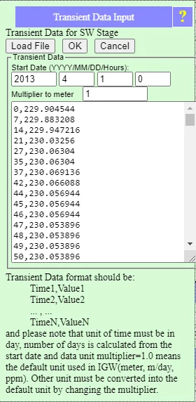
16.3.2 Land Use and Cover tab — Manning's coefficient
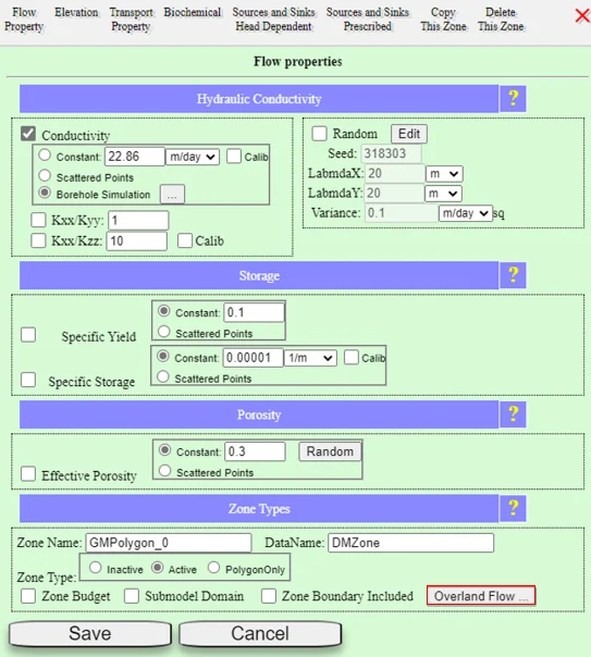
Land Use and Cover configures the surface roughness field — how much resistance each cell offers to overland flow. Manning's n values range from ~0.02 (smooth concrete, glossy surfaces) to ~0.5 (dense vegetation, forested wetlands). Typical ranges by land cover:
- Urban impervious — 0.013 to 0.020 (very smooth, fast overland flow)
- Residential lawn — 0.15 to 0.25 (moderate roughness)
- Cropland — 0.03 to 0.06 (relatively smooth; varies with crop)
- Grassland / pasture — 0.15 to 0.40 (rough due to vegetation)
- Forest — 0.40 to 0.80 (very rough due to understory and litter)
- Wetlands — 0.35 to 0.80 (high roughness from vegetation in shallow water)
The Data Center auto-populates reasonable defaults per land cover class; for most modeling, these are adequate starting points. Site-specific overrides make sense for specialized land uses (managed agriculture, restored wetlands) or when calibration indicates the defaults aren't matching observed runoff timing.
16.3.3 Climate tab — rainfall and evaporation
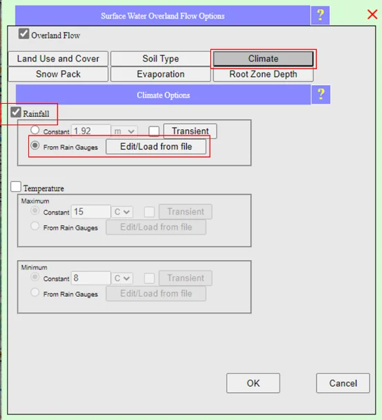
The Climate tab configures:
- Rainfall source — From Data Center (preferred; NLDAS, PRISM, or regional equivalents at the appropriate resolution), Rain Gauges (specific gauge records), or user-uploaded files. Rain is distributed spatially across the domain; temporal resolution depends on the source.
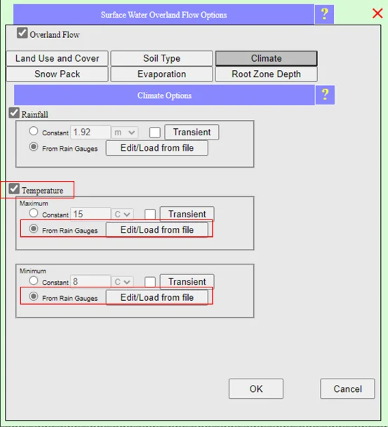
- Temperature — needed for snow accumulation/melt computations and for ET calculation. From Data Center auto-populates from NLDAS or PRISM.
- Evaporation / evapotranspiration — pan evaporation, calculated PET from temperature, or user-specified. Drives water removal from soil moisture and lake surfaces.
- Seasonal rainfall patterns — IGW-NET's Watershed Solver supports four seasons (Summer, Fall, Winter, Spring), each with a configurable hours-per-day and date range. This captures seasonal variability without requiring a full climate time series.
The seasonal rainfall configuration is worth highlighting because it's distinctive:
| Season | Typical configuration | Example |
|---|---|---|
| Spring | Moderate rainfall, multiple hours/day | March 20 – June 20, 4 hours/day |
| Summer | Intense shorter events | June 21 – September 20, 2 hours/day |
| Fall | Moderate rainfall, longer duration | September 21 – December 20, 3 hours/day |
| Winter | Snow-dominated (handled by snow routine) | December 21 – March 19, mostly snow |
Each season's hours-per-day and date range is configurable; the default values are tuned for a Michigan-type temperate climate, so adjust for arid regions, tropical regions, or Southern Hemisphere locations.
16.3.4 Soil Type tab — infiltration parameters
The Soil Type tab configures how water moves into and through the soil column:
- Soil raster — spatial distribution of soil types across the domain. From Data Center (STATSGO for continental-scale, SSURGO for US-detailed, equivalent elsewhere), user-uploaded raster, or constant.
- Lookup table — per soil type, parameters including:
- Saturated hydraulic conductivity (Ksat) — controls how fast water infiltrates once pores are saturated
- Field capacity — soil moisture level below which water is held against gravity (not drained to GW)
- Wilting point — soil moisture level below which ET extraction ceases
- Soil storage capacity — total water the soil column can hold between these thresholds
- Porosity — void fraction; governs the maximum saturation level
- Initial conditions — initial soil moisture state (Cta0000 files in transient simulations, setting the starting soil storage per cell)
These parameters together govern the partitioning of rainfall between infiltration, runoff, and ET — the core computation of the Watershed Solver.
16.4 The Manning's n Gotcha — Stored Everywhere, Active Only When the Solver Is On
A recurring source of confusion in IGW-NET modeling: Manning's coefficient appears in many feature attribute dialogs — polyline attributes, zone attributes, land use classifications. It looks like a universal parameter. But it is only active when the Watershed Solver is enabled.
16.4.1 Where Manning's n appears in IGW-NET
Manning's coefficient is stored as an attribute on:
- Polyline features — streams, rivers, drains, and canals; Manning's n is a per-polyline attribute visible in the Polyline Attributes dialog (Ch. 6 §6.3 and Ch. 14 §14.3.4)
- The Server River Options defaults — per stream-order row in the Order Based table (Ch. 14 §14.6.4, Fig. 14.11); defaults range from 0.045 for small channels to 0.025 for major rivers
- Land Use and Cover classifications — per land-cover class (Fig. 16.2); values from 0.013 (urban) to 0.80 (forest)
- Zone feature attributes — for zones representing lakes, reservoirs, or wetlands
The presence of Manning's n everywhere suggests it is a core simulation parameter. It is — when the Watershed Solver is active.
16.4.2 Why Manning's n is a Watershed-Solver parameter
Manning's n appears in the hydraulic equations governing open-channel flow and overland flow — specifically in Manning's equation: Q = (A × R2/3 × S1/2) / n, where Q is discharge, A is cross-sectional area, R is hydraulic radius, S is slope, and n is Manning's coefficient. These equations are only invoked when water is routing across the surface or through a channel — which only happens when the Watershed Solver is computing surface routing.
The Ch. 14 Level-2 head-dependent flux equation, Q = leakance × (hsw − haq), does not involve Manning's n at all. Whether a stream is a one-way drain or two-way stream, whether a lake is gaining or losing, whether the aquifer drains to the DEM surface — none of these computations use Manning's coefficient. Manning's n only enters when the Watershed Solver is computing actual flow of water across surfaces and through channels.
16.4.3 The symptom and the fix
This is the most common Manning's-n symptom. A user opens a polyline attribute dialog, modifies Manning's n (expecting faster or slower stream response), re-simulates, and sees no change in the aquifer heads or SW fluxes. The reason: the Watershed Solver is not enabled, so Manning's n is stored metadata not affecting the simulation.
The fix depends on what you actually want:
- If you want Manning's n to affect the simulation → enable the Watershed Solver in Simulation Settings. Then Manning's n becomes a real parameter controlling overland and channel flow routing.
- If you're trying to affect stream-aquifer exchange rates → change the leakance, not Manning's n. Leakance controls the Ch. 14 head-dependent flux; Manning's n does not.
- If you're trying to affect overland flow velocity → you need the Watershed Solver active; Manning's n alone without the solver does nothing.
The confusion is structural, not user error — IGW-NET stores Manning's n universally because the attribute is part of the feature's complete data model, but the parameter only activates under specific solver conditions. Recognizing this distinction is part of understanding how IGW-NET's modular solver architecture works.
16.5 Coupling with Coupled Lakes — The Runoff Delivery Mechanism
Chapter 15 introduced coupled lake-aquifer modeling with a lake water balance tracking Ins (precipitation, runoff, SW inflow, gaining GW flux) and Outs (evaporation, SW outflow, losing GW flux). The Runoff In is where the Watershed Solver fits into coupled-lake modeling.
16.5.1 How runoff reaches a coupled lake
When both the Watershed Solver and a coupled lake (Level-3 "From coupled SW/GW modeling") are active, the coupling is automatic:
Rainfall hits the watershed around the lake
Rainfall rate from the Climate configuration (raster, gauge, or user-specified) applies to every cell in the domain, including cells outside the lake polygon.
Rainfall partitions into infiltration and runoff
Soil type (Soil Type tab) and slope (from DEM) determine how much infiltrates and how much runs off. Infiltrated water may become recharge; runoff continues as surface water.
Runoff routes across the land surface
Overland flow follows topography, governed by Manning's n (Land Use and Cover tab). Water flows toward topographic lows — including toward any lake polygons in the domain.
Runoff reaching the lake polygon is added to the lake water balance
Automatic. No CSV import, no manual specification. Every time step, the total runoff entering the lake polygon from the surrounding watershed is computed by the Watershed Solver and appears as the "Runoff" In in the lake balance (Ch. 15 §15.2.2).
Lake stage updates per Ch. 15's water balance
The Runoff In enters alongside Precipitation, SW Prescribed Source/Sink, and gaining GW flux. Outs (Evaporation, SW outflow, losing GW flux) are subtracted. Net storage change → new stage via bathymetry.
If you are building a coupled-lake model (Ch. 15 Level 3) for a natural lake with a meaningful contributing watershed — the lake receives runoff from a surrounding drainage area — you likely need the Watershed Solver (Ch. 16). Without it, Ch. 15's runoff In must be specified manually (SW Prescribed Source/Sink with a runoff time-series CSV) or omitted entirely. Omitting runoff typically underestimates Ins, producing lake stages that drift downward unrealistically. Manual specification requires you to know the runoff time series — which usually means you ran a separate watershed analysis anyway.
Exceptions where you can skip the Watershed Solver for a coupled lake:
- Urban lakes with piped stormwater — runoff is captured by infrastructure before reaching the lake; the natural watershed contribution is near zero
- Reservoirs fed by controlled inlets — water entry is dominated by engineered releases, specified via SW Prescribed Source/Sink
- Short-duration simulations where seasonal rainfall averages out and static recharge is adequate
- Models where you're importing SwaNET-computed recharge via server exchange — the basin-scale runoff is already in the recharge field (§16.6)
16.5.2 The Barron Lake example
The Barron Lake case study (Ch. 15 §15.4, full walkthrough in the case-studies section) uses both the coupled-lake framework and the Watershed Solver together. The specific configuration:
- Coupled lake — "From coupled SW/GW modeling" enabled; bathymetry via WaterDepth.txt; augmentation pumping via SW Prescribed Source/Sink (Qsw.csv)
- Watershed Solver — enabled in Simulation Settings; Land Use and Cover from Data Center; Climate with Data Center rainfall and temperature; Soil Type from Data Center SSURGO raster
- The coupling — runoff from the ~4 km² watershed around Barron Lake routes into the lake automatically; combined with direct precipitation on the lake, SW augmentation, and GW fluxes, the full water balance is complete
The 135-day transient run produces lake stages, aquifer heads, and a complete itemized water balance — all Ins and Outs tracked through time, all responding to the actual rainfall events in the climate data.
16.6 SwaNET — The Two-Platform Architecture for Full Basin Modeling
The IGW-NET Watershed Solver is a subsystem inside IGW-NET. SwaNET is a platform unto itself. They are two points on the same integrated SW-GW modeling spectrum, designed to work together for projects where watershed fidelity matters more than a single platform can serve.
16.6.1 What SwaNET is
SwaNET is MAGNET4WATER's watershed modeling platform, built on USDA's SWAT (Soil and Water Assessment Tool) engine. It is designed for watershed-primary modeling — basin-scale hydrology, agricultural water management, nutrient and sediment transport, reservoir and water-supply studies, land-use scenario analysis. SwaNET brings to MAGNET4WATER the same global base model and AI-assisted interactive experience as IGW-NET, but with SWAT's full watershed physics instead of groundwater.
Where IGW-NET's Watershed Solver has modest-scope watershed processes suitable for GW coupling, SwaNET has the complete watershed treatment: detailed soil layers, plant growth simulation, management practices, tile drainage, stream-order-specific routing, point and non-point source loading, multi-year climate forcing. The standard toolkit that watershed practitioners expect.
16.6.2 The integration architecture
SwaNET sees the basin. Full watershed scope, SWAT physics, basin-scale outputs (streamflow, nutrient loads, sediment yields, reservoir balances, agricultural water budgets).
IGW-NET sees the aquifer. Full groundwater scope, MODFLOW / IGW physics, aquifer-scale outputs (hydraulic heads, velocities, capture zones, contaminant plumes, well yields, lake-aquifer coupling).
They share the domain. The watershed boundary is the same object in both platforms, not two different representations. Shared grids, shared DEM, shared hydrography — one domain, two perspectives.
Recharge fields transfer seamlessly via server exchange. SwaNET computes what reaches the aquifer across the shared watershed boundary. IGW-NET receives it as a dynamic recharge input. The interface between them is a clean data exchange, not a duplicated model.
Surface truth meets subsurface truth. Each platform brings its own rigor; together they form an integrated SW-GW system that neither platform alone could model.
16.6.3 Projection requirements — the UTM handshake
Server exchange between SwaNET and IGW-NET is not just a conceptual data flow; it has specific technical requirements around coordinate projection. SwaNET exports its recharge output in UTM projection; IGW-NET must be set to match. Getting the projection right is the practical difference between a working handshake and a silently-broken coupling.
Why projection matters here
MAGNET4WATER's default display uses a geographic or Web Mercator coordinate system for the interactive map experience — convenient for zooming around the globe and overlaying hydrography, but not suitable for cell-to-cell numerical data transfer. Hydrologic calculations and spatial data exchange need a projected coordinate system with real-world units (meters), where a cell of "30 m × 30 m" actually means 30 meters on each side regardless of where on Earth the domain sits. UTM (Universal Transverse Mercator) is the standard choice for projected coordinates at regional modeling scales.
SwaNET's watershed computations run on UTM grids. Its recharge output is exported in UTM coordinates. For IGW-NET to receive that recharge correctly — with cells aligned to the SwaNET basin — IGW-NET must also be operating in UTM, using the same UTM zone and datum as the SwaNET model.
The configuration steps
Set IGW-NET to UTM-only mode before importing
Navigate to DomainAttr → Miscellaneous and check "UTM Only". This tells IGW-NET to operate exclusively in UTM coordinates for this model — all grid computations, cell positioning, and data imports will use the UTM projection. Do this before importing recharge or any other SwaNET output; setting UTM mode after data is already loaded can cause projection mismatches that propagate through the model.
Verify the UTM zone and datum
The PRJ file in IGW-NET must match SwaNET's UTM zone and datum exactly. UTM has 60 zones worldwide (Zone 1 through Zone 60), each spanning 6° of longitude; a model in southern Michigan (Barron Lake, for example) sits in Zone 16N on the NAD83 datum. A model in Arizona sits in Zone 12N. The wrong zone puts everything in the wrong place; the wrong datum introduces offsets of tens to hundreds of meters.
Verify in both platforms: SwaNET's export metadata and IGW-NET's active projection should show the same zone and datum. If they don't match, resolve the mismatch before proceeding.
Import recharge via "From SW Model Output"
In IGW-NET, when configuring the recharge input, select "From SW Model Output" as the source (rather than Const, Data Center raster, or user file). This tells IGW-NET to load recharge from SwaNET's exported output. Choose the correct file — typically a time-stamped recharge field for the simulation period you're modeling.
Verify alignment before simulating
After import, inspect the recharge field overlay on the model domain. Does the spatial pattern align with the expected watershed drainage? Does the coverage match the domain extent? Spot-check a few cells against the SwaNET output — the same geographic location should show the same recharge value in both platforms. If things look shifted, rotated, or stretched, the projection is likely off; return to the zone/datum verification step.
If IGW-NET is not set to UTM-only mode and you import SwaNET recharge, the import typically still succeeds — IGW-NET applies the data to cells, but those cells may be in the wrong place relative to the SwaNET basin. Symptoms:
- Recharge appears shifted tens of meters to hundreds of meters from where SwaNET produced it
- The spatial pattern of GW heads develops features that don't align with real watershed topography
- Water balance looks numerically fine because the total recharge volume is correct — it's just applied in the wrong places
- Well calibration fails in systematic patterns (some wells always over-predicted, others always under-predicted) that trace back to recharge misalignment
Like the 10×-rainfall pitfall in Ch. 14 §14.7, the signature is a model that looks plausible but is wrong in a specific, traceable way. The fix: confirm UTM mode, confirm matching zone/datum, re-import. Do this once, verify once, and the handshake becomes reliable for subsequent runs.
When to do the projection setup
Set UTM-only mode and confirm projection compatibility:
- Once, at the start of a new IGW-NET model if you know SwaNET coupling will be part of the project
- Before the first SwaNET recharge import if coupling is introduced later
- After any major domain modification that might change the projection context — resizing, moving, or re-georeferencing the model
- When diagnosing unexpected spatial patterns in an existing coupled model — projection mismatch is a common culprit
Users new to MAGNET4WATER sometimes underestimate this step because the default map experience "just works" without explicit projection management. SW-GW coupling, unlike single-platform modeling, requires the projections to be explicit. Thirty seconds of setup prevents hours of troubleshooting.
16.6.4 When to use which
| Project characteristic | Right tool | Why |
|---|---|---|
| GW-primary project, simple watershed coupling needed | IGW-NET Watershed Solver | In-platform subsystem is sufficient; no need to maintain a separate SwaNET model |
| GW-primary project, but watershed complexity is high | SwaNET + IGW-NET via server exchange | Let SwaNET handle the watershed at full fidelity; IGW-NET receives recharge and models the aquifer |
| Watershed-primary project, GW response is secondary | SwaNET (IGW-NET optional) | SwaNET has the full basin treatment; GW modeling can be minimal or omitted |
| Nutrient / sediment / agricultural modeling | SwaNET | Out of scope for IGW-NET; SWAT is the established tool |
| Coupled surface-subsurface analysis (basin-scale) | SwaNET + IGW-NET coupled via server exchange | The integration is the point; both platforms contribute their strengths |
| Regulatory modeling requiring specific watershed-scale outputs | SwaNET | SwaNET produces the standard watershed deliverables expected by regulatory agencies |
16.6.5 The upgrade path
A project can start with IGW-NET's Watershed Solver and escalate to SwaNET coupling later if the watershed side grows in importance. The transition is architectural, not a rewrite:
- The shared global base model means the watershed boundary is already consistent between platforms
- Hydrography, DEM, and climate data are the same in both
- Land use and soil classifications transfer directly
- What changes is where the watershed computation runs — IGW-NET's in-platform solver vs. a SwaNET model with server exchange
This is why neither tool is a dead-end. Start simple; escalate when the project demands it. The architecture expects this escalation and supports it without forcing you to rebuild your modeling work.
16.6.6 A note on access
The Watershed Solver is a premium-tier feature in IGW-NET. SwaNET itself is also a premium platform. The free MAGNET4WATER tier provides:
- Full IGW-NET core modeling — Level-1, Level-2, and Level-3 (coupled-lake) with pre-computed recharge from the Data Center
- Data Center access (DEMs, hydrography, soil rasters, climate rasters from NLDAS/PRISM/HydroSHEDS)
- Global Base Model everywhere on Earth
- AI assistants for model building and interpretation
Premium tiers add:
- IGW-NET Watershed Solver (this chapter)
- SwaNET platform access
- Server exchange between platforms
- Advanced calibration, stochastic simulation, and other specialized features (covered in later chapters)
For current pricing and tier details, see magnet4water.net/Services.
To go deeper
- Chapter 14 — Surface Water as Boundary Conditions — the non-Watershed-Solver baseline treatment of SW; Level-1 DEM-drain and Level-2 explicit features; the stream-order rule; the 10×-rainfall pitfall.
- Chapter 15 — Coupled Lake-Aquifer Modeling — the coupled-lake framework the Watershed Solver supplies runoff to; the lake water balance with Ins and Outs; the explicit time scheme.
- Chapter 17 — T-PROGS 3D Geology — realistic aquifer conductivity; the geological side of coupled SW-GW systems.
- Chapter 18 — Calibration with UCODE — calibrating coupled models against observations; especially relevant when Watershed Solver parameters need tuning.
- Case Study: Barron Lake Coupled Model — full end-to-end example using both coupled-lake modeling (Ch. 15) and the Watershed Solver (Ch. 16) together.
- SwaNET platform — MAGNET4WATER's full watershed modeling platform (SWAT-based).
- magnet4water.net/Services — current premium tier options.