The quick read — 60 seconds
- IGW-NET is the groundwater platform within the MAGNET4WATER water-intelligence ecosystem — the flagship of five sister platforms (IGW-NET, SwaNET, StormNET, ConduitNET, DataNET). This manual covers IGW-NET in depth. Free account. No installation. Anywhere on Earth.
- Every session starts from the Global Base Model — a pre-assembled global foundation of terrain, geology, recharge, and climate. Zoom in anywhere and 80–90% of your model is already built; your job is to refine the rest with local data and expertise.
- The platform is for anyone who needs to understand groundwater in a specific place — students, consultants, researchers, regulators, planners, ecologists, water-utility staff, well drillers.
- IGW-NET's strength is the end-to-end, real-time, streaming visual system. Flow, transport, particles, water balance, 3D visualization all update together as animated movies while the solver advances. Industry-standard engines — MODFLOW (6/2005/USG/NWT) and IGW for flow, MT3DMS (multi-species and dual-domain reactive transport), SEAWAT (variable-density flow), and UCODE (automated calibration) — freed from desktops, connected to global data, streaming in real time. The platform is less a calculator than a visual sandbox for groundwater thinking.
- IGW-NET also supports live collaborative modeling — multiple users in different locations edit the same model synchronously, ideal for student teams and distributed consulting. And it runs first-class stochastic Monte Carlo uncertainty quantification using a "never accumulate" architecture — simulate, analyze, visualize, discard — which is what lets the platform run hundreds or thousands of realizations when most platforms can only afford 10 or 20.
- IGW-NET's two major limitations to know up front: (1) its own physics solver models the saturated zone only — but when coupled with external vadose-zone models (USGS INFIL, USDA SWAT, or the SwaNET watershed platform), the overall modeling workflow does capture unsaturated-zone processes including multi-layer soil moisture, evapotranspiration, land-use effects, and infiltration dynamics, with those models' computed recharge feeding IGW-NET as a physically-derived upper boundary flux; and (2) it assumes Darcy's law applies, which is true for most aquifer materials but not for karst conduits, caves, or large fractures at the scale where those features dominate transport (equivalent-porous-medium representations of karst at regional scale may still be defensible — see §1.4 and Chapter 22 §22.4.8). It also skips dedicated heat transport, full discrete-fracture-network modeling, and HPC-scale continental problems. Everything else in typical regional and site-scale groundwater work is in scope.
- This manual teaches you how to use IGW-NET well: Part I gets you started; Part II walks through the core workflow; Part III covers advanced features; Parts IV–V are reference material. Read Part I linearly. After that, use it as a reference.
1.1 What IGW-NET Is
IGW-NET is the groundwater platform within the MAGNET4WATER water-intelligence ecosystem — the flagship of five sister platforms (IGW-NET for groundwater, SwaNET for watersheds, StormNET for urban water and rivers, ConduitNET for water distribution, DataNET for federated data services and fusion). This manual covers IGW-NET in depth; the other platforms have their own documentation, and the MAGNET4WATER website covers the full ecosystem.
Within its domain, IGW-NET lets you build a working simulation of how water moves beneath the land in a place you care about — a watershed, a property, a region where you're considering a well, a site you're studying, a community you're planning for.
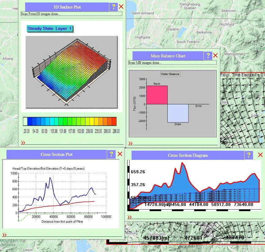
What makes it distinctive is that a working model exists the moment you draw a domain. You do not assemble the model piece by piece before running it. You sketch a rectangle on a web map, and IGW-NET — drawing on the MAGNET4WATER Global Base Model (a pre-assembled global foundation of terrain, geology, recharge, and climate data), typical parameter values chosen for numerical robustness, and a pre-wired solver — immediately has a complete, runnable simulation ready. Often 80–90% of a new model is already built from the Global Base Model; your job is to refine the remaining 10–20% with local data and domain expertise. Click SIMULATE and you see head contours, velocity vectors, a water balance, cross-sections, and 3D views of the water table.
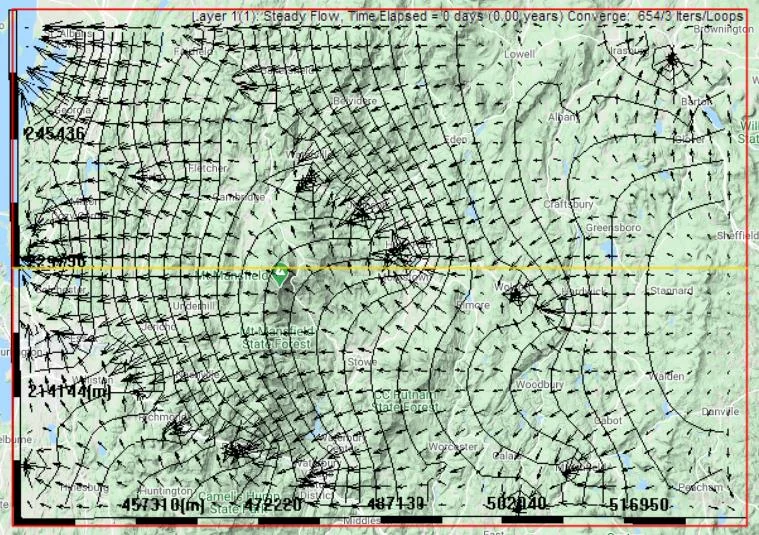
From that starting point — which Chapter 5 calls the base model — you refine. Replace default parameters with your site-specific values. Switch from typical hydraulic conductivity to a Data Center raster specific to your region. Upload your own DEM. Add pumping wells, contamination sources, lakes, streams. Each change is immediately reflected in the visualization. The platform was designed for this refinement-first workflow: you are not "setting up" a model from scratch; you are shaping one that already works.
Under the hood, IGW-NET combines multiple industry-standard solvers into a single unified interface. For groundwater flow, the platform uses the MODFLOW family — MODFLOW-6, MODFLOW-2005, MODFLOW-USG, and MODFLOW-NWT — plus the Interactive Groundwater (IGW) solver for real-time streaming simulation. For solute transport, MT3DMS is integrated with support for multi-species reactions, chain reactions, and dual-domain formulations for fractured or strongly heterogeneous media. For variable-density flow — seawater intrusion, brine migration, thermal plumes — SEAWAT is integrated within the same streaming framework. What users experience on the surface is a map, a drawing tool, a single dialog for aquifer attributes, and a rich visualization stack. The mathematics is handled for you.
The platform is also fundamentally real-time and streaming. Simulations are not static batch jobs — you watch flow fields, plumes, and particles evolve as an animated movie while the solver advances. You can computationally steer the simulation mid-run: change a parameter, add a feature, re-simulate, watch the change propagate. This is why the platform is designed around default-running-then-refining rather than configure-then-run.
IGW-NET makes groundwater visible — so people who need to understand it can, without first becoming software specialists.
1.2 Who Benefits From Using IGW-NET
The platform serves a broad range of users — not because it's generic, but because groundwater affects many kinds of work. Here are the people who most commonly find IGW-NET valuable, and what they use it for.
| If you are a… | You'll likely use IGW-NET to… |
|---|---|
| Student | Complete assignments in hydrogeology courses; explore groundwater concepts in synthetic mode (blank canvas) to build intuition about flow, pumping, transport, and heterogeneity; build models of real places you know; produce figures and analyses for thesis or capstone work — all in a browser. |
| Teaching faculty | Demonstrate groundwater concepts interactively in class using synthetic mode — draw a concept on the blank canvas, watch the physics respond in real time, like a blackboard with live simulation attached; give students a working starting point so they focus on understanding rather than configuration; build reproducible exercises every student can run in a browser. |
| Environmental consultant | Rapidly scope sites in georeferenced mode before committing to detailed investigations; use synthetic mode to test conceptual models and demonstrate "what would happen if…" scenarios to clients; communicate findings with live, editable visualizations instead of static figures. |
| Researcher | Test hypotheses about aquifer response in synthetic mode — heterogeneity effects on transport, regional vertical circulation, coupled dynamics — before investing in a georeferenced model; run comparison studies across sites; prototype ideas before building custom MODFLOW or FloPy workflows. |
| Regulator | Evaluate permit applications by independently reconstructing the applicant's conceptual model (georeferenced mode); test alternative conceptualizations in synthetic mode to see where assumptions matter; assess well interference and wellhead protection proposals on a transparent, shared platform. |
| Planner or ecologist | Understand how land-use changes affect baseflow, wetland hydrology, and groundwater-dependent ecosystems; map where wetlands are expected and how they connect to regional flow; evaluate trade-offs among competing water demands. |
| Water utility or well driller | Screen candidate well sites; estimate sustainable yields; visualize capture zones for public-supply wells; plan wellhead protection areas. |
| Curious person | Understand how groundwater works where you live; use synthetic mode to sketch a concept and see the physics respond; follow public debates about water resources with a working mental model instead of a vague one. |
IGW-NET is equally powerful for georeferenced modeling (a specific site, real data, real coordinates) and synthetic modeling (blank canvas, drawn concept, no real-world tie). A large share of productive use — teaching, scoping, hypothesis testing, concept visualization — happens in synthetic mode. The blank canvas is not a lesser feature; it's a thinking instrument that runs the same physics as the georeferenced case. §1.3.2 covers synthetic mode in depth.
1.3 What IGW-NET Does Well
Four capabilities define the platform. These are where you get real leverage — the things that would take days or weeks of work in other tools and take minutes in IGW-NET.
1.3.1 End-to-end simulation from click one
The moment you define a model domain, a complete, runnable groundwater simulation exists — with aquifer top, bottom, hydraulic conductivity, recharge, porosity, storage, and surface drainage all set to reasonable defaults. You do not configure these before running. You run first, see the solution, and then refine progressively — adding complexity only where it changes the answer. This inversion — from "set up then solve" to "solve then refine" — is the platform's most distinctive design choice, and it reflects a core modeling philosophy: the model guides data collection, the data improves the model, and each iteration is sharper than the last.
And the simulation is not just flow. Add a concentration source and transport activates automatically — you get an animated plume. Drop a zone of particles on the flow field and they animate along the velocity vectors. The water balance is tabulated. Cross-sections colorize themselves. The 3D water table is a single click away.
1.3.2 A visual sandbox — synthetic and georeferenced modes
IGW-NET runs in two modes, and both are first-class. Georeferenced mode is what most of this manual focuses on: you point the platform at a real location, the Global Base Model loads real DEMs, real K rasters, real recharge, real streams and lakes, and you build a model of a specific place. Synthetic mode is the other canonical use — an empty canvas, no real coordinates, where you draw a concept and immediately see what it means. The interface switches you to a blank spot for synthetic work. Both modes use the same solver, the same features, the same visualization. What differs is only whether the domain is tied to real-world geography.
Synthetic mode is not a toy. It is how a large share of serious modeling actually happens — consultants scoping a problem before committing to a full site model, researchers testing a hypothesis about heterogeneity or coupled dynamics, professors teaching the physics of groundwater flow, students exploring concepts as fast as they can think of them. The synthetic canvas is a blackboard with physics attached. What you draw, you simulate. What you change, you see respond. The thinking happens at the speed of sketching.
The workflow is as fast as you think. Draw a domain. Assign a thickness. Set top and bottom elevations however you want — constant, zone-based, scatter-point interpolated, or as a raster (the same tools work as in georeferenced mode). Drop a constant-head polyline representing a fully-connected river on one side. Add a pumping well. You already have a complete, running groundwater simulation, and the flow pattern is visible immediately. Add another well — re-run in seconds. Watch the mass balance update. Drop in particles. See them migrate along flow lines, tracing paths forward from a source or backward from a well to show the capture envelope.
Add a zone of low K. The flow field re-organizes around it in real time, and the particles navigate around the barrier just as they would in the field. Turn on spatially correlated random-field heterogeneity around a mean K (Ch. 19 §19.3) — the effect on transport is dramatic and immediate. The plume stretches, fingers, channels along preferential pathways. You see the small-scale heterogeneity producing the large-scale spreading that theory calls field-scale or macrodispersion (Ch. 19 §19.7.4) — not as an abstract parameter in a textbook equation but as the visible, nonlinear, unmistakable consequence of K structure. The regime demands the grid resolve the correlation scale of the random field, so a refined grid or submodel is usually warranted (Ch. 13) — but that's a few clicks.
Introduce plume sources — from a river reach, from injection, from a leaking lagoon. Flip retardation on. Adjust velocity by moving a boundary. Each change is a fresh simulation that costs seconds, not hours.
Cross-section work is equally direct. You can draw a profile and model it with the same governing equation that applies in plan view. In the vertical profile, anisotropy (horizontal K ≫ vertical K in most aquifers) usually cannot be ignored — but if you vertically exaggerate the profile by the transform factor √(Kx/Kz) the profile becomes effectively isotropic in the transformed coordinate, which is why modelers routinely display vertical sections with that exaggeration. You can also draw a curved upper boundary representing a water table. The water table is, by definition, the surface where pressure equals zero, so water-table head equals elevation — in two dimensions, head = y. IGW-NET lets you assign head = y along a drawn boundary to represent an actively-shaped water table. You see regional vertical circulation emerge from the topography of that boundary in real time. Draw a sloping water table and Tóth's regional-flow patterns appear — local, intermediate, and regional flow cells stacked vertically. Draw a wavy, sinusoidal water table representing topographic relief, and the nested flow systems appear just as in the classic papers. Add an internal horizontal layer of contrasting K — a high-K basal sand unit, or an intermediate low-K aquitard — and you see extended Tóth behavior: water self-optimizes its pathways through the structural geology, routing preferentially through high-K zones, pooling above aquitards, and producing the complex recharge-to-discharge patterns that real glaciated aquifers exhibit.
This prescribed-water-table approach is unmatched for visualizing flow geometry, but it has an important limitation — the simulated fluxes are only physically realistic when the drawn water table and the assigned K field are mutually compatible with available recharge. A steep water table paired with high K will produce enormous fluxes that could not possibly be supplied by rainfall. When flux realism matters — for water-budget analysis, recharge estimation, or site-specific inference — use the 3D-slice approach instead: a narrow one-cell-wide plan-view strip with full vertical resolution, the DEM as the top, and recharge as the input; the water table then emerges as a solution that is by construction consistent with rainfall. Chapter 10 §10.2 covers both approaches in depth, including when to use each.
Used this way, the platform is a thinking instrument. The time from question to insight collapses. Visualizing what heterogeneity does to transport, what a sloping water table does to regional flow, what a pumping well does to a coastal lens — each takes minutes, often less. The physics is not simplified; it is the same governing equations and numerical schemes that run in the georeferenced case. What synthetic mode removes is the data-preparation overhead, so that the full attention can go on the concept.
Entering synthetic mode: From the main IGW-NET interface, click Utilities → Go to Synthetic Case Area. The platform switches from map-based mode to a blank rectangular canvas with no geographic context. This is the single authoritative entry point. (Realtime help: utilities.)
Building a minimal synthetic model from the blank canvas:
- Define domain geometry. The synthetic area starts as a rectangle. Use Draw Domain to reshape if you want a non-rectangular conceptual region. (Realtime help: draw-domain, domain-draw.)
- Set aquifer properties. Click DomainAttr to open the Default Model Input Parameters window. In synthetic mode the Data Center defaults do not apply, so you assign uniform values directly: Hydraulic conductivity (e.g., 35 ft/day), Recharge (e.g., 0 in/year to isolate boundary-driven flow, or a realistic recharge rate), Top elevation and Bottom elevation (constant values for a flat horizontal aquifer). See Chapter 5 for the full customization ladder — the same tools (constant, zone-based, scatter-point interpolation, uploaded raster) work in synthetic mode; only the auto-loaded Data Center defaults are absent.
- Add boundary conditions. Draw constant-head polylines along the sides to represent regional flow direction. Or draw river/drain polylines with leakance for head-dependent boundaries. See Chapter 6 for feature tools and Chapter 14 for surface-water BC details.
- Add wells and sources. Click Draw Well to place pumping, injection, or monitoring wells. Set pumping rate, screen intervals, and (for transport) concentration. (Realtime help: draw-well.)
- Simulate. Click Simulate. The solver runs and you see heads, velocities, and mass balance immediately. Iterate: change a parameter, re-simulate, observe.
- Add particles or transport. Use Particle Tools for forward/backward tracking (Chapter 11). Define a concentration source to activate transport automatically (Chapter 12).
- Turn on heterogeneity. In the attribute dialog, enable random-field generation on K (or any supported property). Set the mean, variance, correlation scales (
LambdaX,LambdaY,LambdaZ), and a seed. See Chapter 19 §19.3 for the full random-field setup. Important: to resolve macrodispersion visibly, the grid must resolve the correlation scale — add a refined submodel (Chapter 13) or increase NX/NY so that at least 5–10 cells fit within one correlation length.
Tutorials to work through — all ready-made for synthetic mode:
- Tutorial 9 — Synthetic Heterogeneous Aquifer Model. The canonical synthetic-mode walkthrough. Starts with "Click Utilities → Go to Synthetic Case Area" and builds up through uniform properties, boundary conditions, random-field heterogeneity, and calibration against a "known" subsurface. Read this first if you want a complete end-to-end synthetic example.
- Tutorial 6 — Vertical Flow Dynamics. Sublayer resolution, recharge and discharge zones, regional vertical circulation. Often done synthetically first to build intuition.
- Tutorial 12 — 2D Cross-Sectional Profile Modeling. The vertical-profile workflow for Tóth flow, saltwater intrusion, and density-driven problems. Combined with the
head = ywater-table boundary technique, this is where you reproduce the classical regional-flow figures. - Tutorial 20 — Theis Solution for Pumping Test Analysis. Build an analytical-solution benchmark in synthetic mode and verify IGW-NET against a closed-form result.
- Tutorial 15 — Single-Realization Stochastic Flow. Spatially correlated random-K field, observe heterogeneity effects on heads and flow — the foundation for seeing macrodispersion emerge.
- Tutorial 17 — Monte Carlo Transport. The ensemble treatment of transport under K uncertainty. Macrodispersion as an ensemble-mean phenomenon.
- Tutorial 3 — Particle Tracking. Forward and backward particle tracking — works in synthetic mode identically to georeferenced.
- Tutorial 5 — Contaminant Transport. Advection, dispersion, and reactions. Start synthetic to isolate transport physics before adding site-specific complexity.
Quick-recipe: reproducing the Tóth regional-flow figure in minutes. Enter synthetic mode → draw a wide-and-shallow rectangular domain (cross-section orientation) → set K uniform, recharge = 0 → assign no-flow sides and bottom → along the top boundary, draw a polyline with head = y (follows a sinusoidal or sloping elevation you define) → mark the region above the water-table line as Inactive → simulate. The local, intermediate, and regional flow cells appear stacked vertically. Add particles along the top surface to visualize residence times across the flow-system hierarchy. Flux-realism check: the simulated discharge should be compared against (domain area × a plausible recharge rate, e.g., 10 in/year for glaciated mid-latitude climate). If the simulated flux exceeds this by more than ~2×, your water table is too steep for the K you chose — reduce one or the other. Ch. 10 §10.2 explains the compatibility constraint.
Quick-recipe: extended Tóth with structural geology. Start from the Tóth setup above → add an internal rectangular zone of contrasting K (for example, a high-K basal sand unit at 3–5× the background K, or an internal low-K aquitard at 1/10 the background) → simulate. The flow field re-organizes dramatically: water routes through the high-K layer, is deflected by the aquitard, and the classical Tóth cells deform into the more complex patterns characteristic of real glaciated aquifers with layered glacial drift. Compare with and without the contrasting layer to see how structural geology redirects the natural recharge-to-discharge pathways.
Quick-recipe: physically-consistent vertical profile via 3D slice. For cases where flux realism matters (e.g., recharge estimation, water-budget analysis, real-site interpretation), build a one-cell-wide 3D slice instead. Stay in georeferenced mode → draw a narrow rectangular domain through the area of interest (one cell wide in plan view) → accept the Global Base Model DEM as the top → declare multiple conceptual layers corresponding to your hydrostratigraphy, each with its own K and internal sublayers → recharge is applied from the Data Center (default) or as a specified rate → simulate. The water table is not prescribed; it emerges as part of the solution, automatically consistent with the recharge flux. Display a cross-section along the slice to see the vertical flow structure with guaranteed water-balance closure. Particularly revealing in glaciated terrain (Michigan-style): the DEM-driven topography, real K structure, and realistic recharge produce a vertical profile whose circulation patterns are close to what the real aquifer does. See Tutorial 6 for a worked Michigan example.
Quick-recipe: visualizing macrodispersion from heterogeneity. Enter synthetic mode → draw a rectangular domain → assign constant-head boundaries on left and right (uniform gradient) → enable random-field K with a specified mean, variance of 1 (lnK), and correlation length Lambda ~1/20 of the domain width → set grid resolution so at least 5–10 cells fit within one Lambda → add an instantaneous contaminant source as a small zone at the inflow boundary → simulate. The plume stretches, fingers, and spreads along preferential flow paths. Toggle random-field off (uniform K) to compare — the difference is the macrodispersion signal. Run ensemble Monte Carlo (Chapter 19 §19.5) to quantify it statistically.
1.3.3 Data Center and DataNET — no GIS wrangling
A library of curated spatial datasets is built into the platform. Hydraulic conductivity rasters for Michigan, the USA, and globally. Bedrock elevation. Long-term mean recharge. DEMs at 1 m, 10 m, 30 m, and 90 m resolution. Precipitation and climate data. Static water levels from dense statewide water-well databases. USGS sensor data for transient calibration. Borehole lithology data for 3D geologic modeling. Instead of downloading, reprojecting, and clipping each layer, you pick from a dropdown. The platform handles the spatial operations behind the scenes.
Beyond the built-in Data Center, IGW-NET includes a direct bridge to DataNET web services — WMS, WFS, and WCS layers organized by region and environmental category in a multi-scale Data Tree. You can also import from external or third-party web data servers, making any OGC-compliant data source available for model parameterization. And when you have better local data than any online service offers — site-specific K from aquifer tests, project-specific recharge, custom borehole logs — you upload your own raster, shapefile, or borehole logs, and the platform uses your data in place of the defaults.
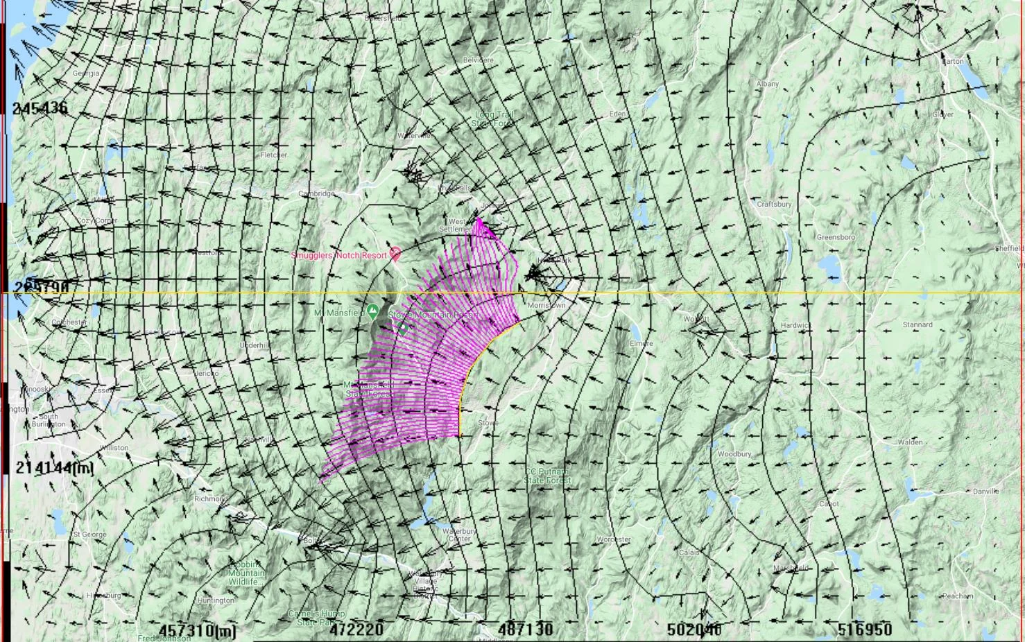
A particularly powerful example of the DataNET architecture is LiDAR DEM delivery. LiDAR coverage for all of North America is available from USGS WMS/WCS services, but LiDAR datasets for any sizable region are genuinely massive — impossible to move as local files, and difficult to handle in platforms that require manual DEM preparation. IGW-NET resolves this by streaming LiDAR through DataNET on demand, with automatic subsampling by area: for a large regional domain, the subsampled resolution is appropriate to the grid; for a small local domain, the original 1 m resolution is preserved. The model file stays light because the data stays virtually immobile on the server. Combined with hierarchical modeling (Chapter 13), this means a regional parent model with standard DEM and a fine-resolution submodel with LiDAR over an area of interest is a practical everyday workflow rather than a data-management project. It's one of the concrete ways the platform removes logistical barriers that would otherwise limit what a single modeler can do. A flagship application is headwater groundwater-dependent ecosystems — fens, hanging bogs, coldwater headwater reaches, wetland complexes where small topographic features control where groundwater emerges and which wetlands are GW-fed. Classical workflows with 10 m or 30 m DEM cannot resolve the topography that controls discharge in these settings; LiDAR with hierarchical modeling makes the modeling tractable, and Chapter 22 §22.2.5 develops this in detail. The customization ladder (Chapter 5) formalizes how this progressive refinement works.
1.3.4 Instant local refinement via submodels and unstructured grids
When regional resolution isn't enough for a specific question, you don't rebuild the model at a finer grid. You draw a box inside the parent domain, check "Boundary Condition from Parent Model," and you have a refined local model whose boundaries inherit from the regional solution. The whole operation takes about a minute. Chapter 13 covers this in depth; the point for now is that local refinement in IGW-NET is a one-minute operation, not a multi-day rebuild.
When refinement needs are even more specific — a pumping well, a stream, a small plume source — IGW-NET also supports unstructured grids: rectangular cells of varying size, with refinement concentrated where head or concentration gradients change rapidly. You can generate refinement zones inside the platform, or import them from an external shapefile. Unstructured-grid results display on the same map and feed the same cross-section, water balance, and particle-tracking tools as structured-grid results. See Chapter 19 for the MODFLOW 6 DISV path that powers this.
1.3.5 Reactive transport, variable density, and multi-species
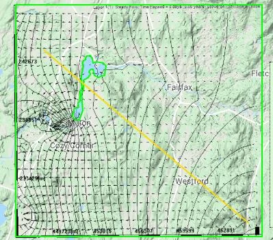
Transport in IGW-NET is not limited to simple conservative tracers. The platform integrates the industry-standard MT3DMS transport solver with support for:
- Multi-species reactive transport — track multiple interacting solutes simultaneously, including parent-child chain reactions (PCE → TCE → DCE → VC sequential degradation), interspecies reactions (electron donor / electron acceptor coupling), and predefined modules for common contaminants like BTEX (aerobic and multi-electron-acceptor kinetic decay pathways).
- Dual-domain transport — a mobile-domain / immobile-domain formulation that handles slow-tailing plumes in fractured rock, macroporous soils, and strongly heterogeneous aquifers where single-domain models fail. This is IGW-NET's effective approach to representing fractured-media transport without requiring a dedicated discrete-fracture-network solver.
- Variable-density flow and transport via the integrated SEAWAT engine. Saltwater intrusion in coastal aquifers, brine migration from injection wells or evaporite dissolution, and thermal plumes from geothermal or industrial sources all run within the same streaming framework as standard flow.
All of these run in the same end-to-end pipeline as the base model — plumes animate in real time, concentration breakthrough at monitoring wells is charted as the simulation advances, and you see both head and concentration fields updating together. Chapters 11 and 12 cover transport in depth.
1.3.6 Stochastic and uncertainty quantification
Real aquifers are heterogeneous at scales smaller than any grid can resolve. IGW-NET addresses this with built-in stochastic tooling — not as an afterthought, but as a first-class capability. Two complementary approaches:
- Sequential Gaussian Simulation (SGS) — generates spatially correlated random K fields with user-controlled mean, variance, and correlation structure. IGW-NET runs full Monte Carlo simulations across hundreds or thousands of realizations, computing ensemble statistics on the fly: mean head and plume fields, variance maps, probabilistic capture zones, probability of MCL exceedance at monitoring points, and live-streaming hydrographs across realizations. This is made possible by the platform's never-accumulate architecture (see callout below).
- Transition Probability (T-PROGS) geostatistics — generates discrete geologic realizations from borehole records, with multiple material categories (e.g., aquifer / marginal-aquifer / partially-confining / confining) each with characteristic K values. For T-PROGS, users simulate one realization at a time; ensemble analysis is manual rather than automatic.
Monte Carlo forward and reverse particle tracking generates probabilistic capture zones and influence zones. Together these tools move IGW-NET from deterministic single-answer modeling to risk-based, uncertainty-aware prediction. Chapter 18 covers stochastic modeling in depth.
IGW-NET operates on one architectural principle across Monte Carlo, transient flow, particle tracking, and transport: simulate, analyze, visualize, discard. Running ensemble means, variance maps, and exceedance probabilities are updated on the fly as each realization completes; the realization itself is then discarded. Memory usage stays constant regardless of how many realizations or time steps you run.
This is not a clever optimization — it is the only architecture that makes serious cloud-native stochastic modeling feasible. The first 80% of ensemble convergence is fast; the final 20% — where the probabilistic tail gets resolved and risk assessments become defensible — takes orders of magnitude more realizations. Most stochastic-modeling platforms settle for 10 or 20 illustrative realizations because they have no way to handle more. IGW-NET runs until the ensemble actually converges because it never accumulates the data it would otherwise choke on.
The same principle applies to transient flow and particle tracking: by default, time snapshots are not preserved across steps. Running statistics (mean, variance, min, max, cumulative fluxes) are maintained; individual time states are streamed to the visualization and discarded. If you need to preserve specific snapshots (for report figures or frame-by-frame analysis), enable saving explicitly for those steps.
1.3.7 Calibration with big data
Calibration in IGW-NET is designed around the reality that most modelers today have access to dense but noisy statewide water-well databases — thousands of static water-level measurements per region, of variable quality. The platform handles this through two integrated paths:
- Manual calibration with multipliers — adjust K or recharge multipliers while watching the calibration scatter plot update in real time. Because multipliers preserve spatial structure while shifting overall level, calibration stays defensible (see Chapter 5 §5.5.4 for why this matters).
- Automated parameter optimization via UCODE — nonlinear-regression inverse modeling (Poeter and Hill, 1999) integrated directly into the platform. Observations to match: heads, fluxes to surface-water bodies, concentrations. Parameters that can be optimized: recharge and K multipliers, anisotropy ratios, specific yield and specific storage, river/stream/lake leakances, and drain leakances. No separate installation, no input file editing.
USGS time-series sensor data can be extracted directly for transient calibration — or used for steady-state calibration by comparing average, maximum, or minimum observed water levels to simulated heads. Chapter 17 covers calibration in depth.
1.3.8 Collaborative modeling — unique among platforms
Because IGW-NET is cloud-native, it enables something that desktop modeling tools cannot: multiple users working live on the same model simultaneously, from anywhere in the world. When you sign up, you are prompted to invite collaborators or add guest accounts; those collaborators can then edit the same domain, zones, features, and attributes you are editing, with all changes visible to every user in real time. When any user clicks SIMULATE, all users see the results simultaneously.
This matters in several contexts:
- Student team projects. Teams no longer need to coordinate schedules around a shared computer lab. Students in different dorms, different cities, or different countries can work on the same model synchronously — typically while on a video conference — just as if they were sharing a laptop.
- Distributed consulting teams. A regional hydrogeologist, a project lead, and a regulatory reviewer can inspect the same model together, in real time, from three different offices.
- Peer learning and mentorship. An instructor can watch a student's work as it unfolds and intervene in real time; a senior modeler can demonstrate techniques to several juniors at once.
This is distinct from asynchronous collaboration through the MAGNET4WATER Observatory (Chapter 2 §2.5), where published models are shared for others to download and extend on their own time. Synchronous collaboration makes IGW-NET a real-time shared workspace, not just a shared library.
1.4 What IGW-NET Doesn't Do
Honest positioning requires being clear about fit. IGW-NET is a broad platform, but it is not universal. Here are the situations where another tool is a better choice.
| If your work requires… | Consider instead… |
|---|---|
| Detailed 1D column unsaturated-zone flow (Richards equation for irrigation return flow through a specific soil profile, tension-saturation curves for a specific soil, pore-scale unsaturated physics) | HYDRUS or VS2D for column-scale Richards-equation work. IGW-NET's own solver treats the saturated zone only, applying recharge as a flux at the water table — but for spatial unsaturated-zone physics (recharge computed from climate forcing, multi-layer soil moisture accounting, evapotranspiration, land-use effects, deep percolation through variable soils), the standard IGW-NET workflow is coupling with external watershed models: the USGS INFIL recharge model, USDA SWAT, or the SwaNET platform within the MAGNET4WATER ecosystem. These produce physically-derived spatial recharge fields that replace the naive “direct-to-water-table” assumption. See Chapter 16 for the SwaNET handshake and coupled-modeling workflow. |
| Discrete-fracture-network modeling (explicit representation of individual fractures) | FracMan or dfnWorks for full DFN work. Note: for effective transport in fractured media, IGW-NET's dual-domain MT3DMS formulation (see §1.3.5) handles the key mass-exchange physics without explicit fracture geometry — this suffices for most practical fractured-aquifer questions. |
| Karst or conduit-flow modeling at the scale where individual conduits and caves matter (turbulent flow, very fast tracer velocities, conduit network hydraulics) | MODFLOW-CFP, CFPv2, or dedicated conduit-flow codes. IGW-NET's Darcy-based continuum formulation can provide a defensible equivalent-porous-medium representation of karst aquifers at regional scale (water balance, broad head distributions), but it cannot capture conduit-scale transport or the rapid storm-response that defines karst behavior. The distinction is scale: EPM in IGW-NET is appropriate for large-scale averaged questions about karst, not for site-scale conduit-aware questions. Chapter 22 §22.4.8 covers this boundary in detail. |
| Dedicated heat-transport modeling for general thermal problems (geothermal systems, thermal energy storage with complex boundary conditions) | SUTRA or HydroGeoSphere for thermal-problem-first work. Note: IGW-NET supports thermal plumes through SEAWAT's variable-density coupling (§1.3.5), which is sufficient for seawater-intrusion and thermal-intrusion problems where temperature affects density. For heat-transport as the primary physics, a dedicated tool is a better fit. |
| Very-high-performance HPC modeling at continental scale with tens of millions of cells | MODFLOW 6 in a dedicated HPC environment. IGW-NET's cloud solver handles most regional and site-scale models comfortably, but at the extreme upper end of problem size, specialized compute is warranted. |
| Specialized MODFLOW packages not yet exposed in the interface (e.g., MNW2 multi-node wells, SFR2 stream routing with full network routing physics, advanced CLN package configurations) | MODFLOW 6 directly, or use IGW-NET's ZipMODFLOW post-analysis tool (§1.3.9) to inspect and visualize externally-built MODFLOW models inside IGW-NET. The platform's own interface covers CHD, DRN, EVT, GHB, RCH, RIV, and WEL packages, with SFR and LAK support coming. |
IGW-NET's own physics solver models the saturated zone only. Above the water table — in the unsaturated or vadose zone — IGW-NET does not itself solve Richards' equation. On its own, it requires recharge to be supplied at the water table as a boundary-condition flux.
In practice, however, this limitation is almost always resolved by coupling. The standard IGW-NET workflow for any model where vadose-zone processes matter is to compute recharge using an external watershed or vadose-zone model and import the resulting spatial recharge field into IGW-NET. Three couplings are routinely used: the USGS INFIL recharge model (which computes infiltration and deep percolation through multiple soil layers with land-use, DEM, soil-property, and ET inputs), the USDA SWAT model (which tracks multiple unsaturated soil layers, runoff, ET, and recharge across a watershed), and the SwaNET platform within the MAGNET4WATER ecosystem (which provides watershed-scale surface-water and vadose-zone physics tightly integrated with IGW-NET through a handshake workflow). These couplings deliver physically-derived spatial recharge — not a flat user-entered value — that accounts for soil moisture dynamics, ET, crop uptake, paved-surface effects, and irrigation return. For most practical IGW-NET work, this is how vadose-zone physics enters the model.
The cases where even coupled modeling isn't sufficient are narrow: detailed 1D column studies requiring Richards-equation-level accuracy for a specific soil profile (use HYDRUS or VS2D), or problems where the vadose zone and aquifer are in such tight feedback that a fully coupled single-code treatment is needed (coupled MODFLOW-UZF). For these cases, the dedicated tools are appropriate. For everything else — the vast majority of regional and site-scale work involving recharge — the coupling with INFIL, SWAT, or SwaNET covers the physics fully.
IGW-NET solves Darcy's equation, which describes flow through a continuous porous medium where velocity is linearly proportional to hydraulic gradient. This assumption holds superbly for sediments, sedimentary rocks, weathered bedrock, and most typical aquifer materials. It breaks down, however, in systems where flow happens primarily through discrete features rather than a porous matrix: karst aquifers with conduits and caves (where flow is often turbulent rather than laminar), aquifers containing major fractures or fault zones with significant aperture, and some fractured crystalline rock settings where transmissivity is concentrated in a sparse fracture network. The subtlety is that Darcy applicability is scale-dependent — a karst aquifer that plainly violates Darcy at the scale of an individual conduit may behave approximately like an equivalent porous medium when observed over large enough regions (kilometers to tens of kilometers), as the collective behavior of many features averages toward something diffusive. Whether this equivalent-porous-medium representation is useful depends on your question: for a regional water-balance study of a karst aquifer, it may be adequate; for predicting contaminant arrival time in a specific well in karst, it is not, because transport in conduits happens in hours to days rather than the diffusive timescales a Darcy model will produce. When you encounter karst features (large-discharge springs, rapid water-level response to storms, sinkholes, cave systems, dye-tracer velocities greater than ~10 m/day), stop and decide: is the EPM approximation appropriate at the scale of your question, or do you need a discrete-fracture-network code or a conduit-flow model instead? Chapter 22 §22.4.8 develops this boundary in detail.
1.4.1 The ZipMODFLOW post-analysis bridge
For externally-built MODFLOW models — whether from another platform, a published study, or a legacy project — IGW-NET offers the ZipMODFLOW post-analysis tool. Load an existing MODFLOW model, run it inside the platform, inspect boundary conditions, draw cross-sections, perform basic calibration, run MODPATH particle tracking, and more. This is how users bridge existing MODFLOW workflows with IGW-NET's visualization and analysis capabilities without rebuilding the conceptual model.
IGW-NET is the right tool for the broad middle of groundwater work — most regional and site-scale flow, transport (including reactive multi-species and variable-density), particle tracking, stochastic uncertainty, and calibration problems. The saturated-zone-only focus is deliberate: it is what keeps the platform fast, accessible, and usable anywhere in the world without local installation. For the genuinely specialized problems listed above, we'll say so in this manual rather than stretching the platform to cover something it's not built for.
1.5 The Core Vocabulary
A set of terms threads through this manual and the MAGNET4WATER ecosystem. Learning them now makes the rest of the manual — and the wider website — easier to follow.
| Term | Meaning | Where you'll see it |
|---|---|---|
| Conceptual model (xyz) | What you build — the real-world domain, zones, wells, polylines, layers, and attributes expressed in continuous xyz coordinates. This is the faithful representation of your site. You can edit it anytime without rebuilding anything. See §1.5.1 below for the fundamental distinction this sets up. | §1.5.1; everywhere |
| Numerical model (ijk) | What the solver sees — the computational grid where each cell has a row (i), column (j), and layer (k) index. Produced by discretizing your conceptual model onto the grid every time you SIMULATE. Always an approximation of the xyz conceptual reality; how good an approximation depends on grid resolution. | §1.5.1; Ch. 7; Ch. 13 |
| Discretization | The xyz → ijk mapping. At SIMULATE time, IGW-NET reads every conceptual feature (your domain, zones, wells, polylines, layers, attributes) and maps them onto the grid to create the numerical representation. Discretization happens every SIMULATE; you do not build or maintain the grid directly — you build and maintain the conceptual model. | Ch. 7 §7.3 |
| Global Base Model | The MAGNET4WATER-level foundation — a pre-assembled global fabric of terrain, geology, recharge, climate, and hydrography, available to every session in every platform. You "zoom in anywhere on Earth and a working model is ready" because 80–90% is already built from this foundation. Distinct from the per-session base model (below). | Ecosystem-level |
| Base model | Your specific, runnable simulation — the one that exists as soon as you draw a domain. Populated from the Global Base Model plus typical defaults. You refine it — you don't build it from scratch. | Ch. 5; everywhere |
| Near-surface, unconfined, water-table aquifer | The shallow aquifer system that the base model represents by default. Where water supply wells, wetlands, springs, and baseflow-driven streams live. | Ch. 5 §5.1.1 |
| Refine progressively | The platform's core modeling philosophy: add complexity only when it changes the answer. The model guides data collection; the data improves the model; each iteration is sharper than the last. Operationalized by the customization ladder (Ch. 5). | Ch. 5 §5.2, throughout |
| Never accumulate | The architectural principle: simulate, analyze, visualize, discard. Running statistics are maintained; individual realizations, time steps, and snapshots are not stored by default. This is what makes serious cloud-native stochastic and long-transient modeling feasible. | Ch. 7, Ch. 18 |
| Observatory | MAGNET4WATER's global network for water intelligence — a unified view of the water system assembled from multiple information sources. Published models from IGW-NET are one element; live sensor feeds from USGS and others, Data Center rasters, and user-contributed data are others. The underlying idea: every model is data, every dataset is a model of reality, and the Observatory lets you see the system using everything available. | Ecosystem-level, Ch. 2 |
| Visual sandbox | Every conceptual-model assumption is editable, every edit is immediately visualized. The model is a living representation of your current understanding, not an artifact you build once. | Throughout |
1.5.1 Conceptual model (xyz) vs numerical model (ijk) — the foundational distinction
More than any other concept in this manual, the distinction between the conceptual model and the numerical model is the idea that unifies how IGW-NET works. Understanding it will make every subsequent chapter click into place.
The conceptual model — what you build in xyz
The conceptual model is your representation of the real-world aquifer system, expressed in continuous spatial coordinates (xyz — longitude, latitude, elevation, or projected equivalents). It includes:
- The domain boundary you drew on the map
- Every zone you added (with its K, recharge, porosity, and other attributes)
- Every polyline you drew (rivers, streams, drains) with their type and attributes
- Every well (pumping or injection) with its coordinates, flow rate, and screen depth
- The conceptual layers representing geologic units
- Any particles you placed for tracking
- Any concentration sources you defined
This is the faithful xyz representation of how you understand the site. Features sit at their real coordinates. A river runs along its true path. A well is at its actual location. Zone boundaries follow the geology as you understand it. This is the model you build and maintain — and the model you can freely edit at any time.
The numerical model — what the solver sees in ijk
The numerical model is a grid-based approximation of the conceptual model. It uses discrete cells indexed by row (i), column (j), and layer (k) — MODFLOW's standard convention. Each cell has one K value, one head value, one concentration value per species, one velocity vector. The solver operates entirely on this ijk representation — solving the flow PDE on the grid, computing cell-to-cell fluxes, integrating through time.
The numerical model is always an approximation of the conceptual reality. A river that traces a sinuous path in xyz becomes a staircase of cells in ijk. A zone boundary that follows a geological contact gets snapped to the nearest cell edge. A particle at some xyz position gets located within a specific ijk cell to determine its velocity. How close the ijk approximation is to the xyz reality depends entirely on grid resolution — which is why this distinction matters.
Discretization — the xyz → ijk mapping, happens at SIMULATE
Every time you click SIMULATE, IGW-NET performs discretization: it reads your conceptual model and maps every feature onto the grid to build the numerical representation. Zones get rasterized onto cells; polylines become sequences of cells; wells get located in their cells; attributes get averaged over cell footprints. This mapping happens completely automatically — you never see or touch the grid directly.
Because discretization happens at SIMULATE time from the current conceptual model, you have a powerful working mode: edit the conceptual model freely, then simulate to see the consequences. The conceptual and numerical models are not linked one-to-one; they are linked by the discretization operation, which repeats every time you simulate.
The xyz–ijk separation is what makes IGW-NET feel the way it does:
- You edit conceptually, not numerically. Move a well by dragging it; the new xyz location gets mapped to the grid at next SIMULATE.
- You can refine progressively. The customization ladder (Ch. 5) is about improving the conceptual model's xyz truth. Better data = better conceptual model = better numerical approximation.
- Particles are light. Once discretization has produced velocities in ijk, particles trace through them without needing re-discretization (Ch. 11 §11.3). That's why Forward/Backward is instant.
- Transport sources force re-SIMULATE. Because concentration sources must be discretized onto the grid before the transport solver can use them, adding a new source requires a fresh discretization pass (Ch. 11 §11.3.4, Ch. 12).
- Numerical dispersion arises from the ijk approximation. Cell-averaging smears the xyz concentration gradients (Ch. 12 §12.4.3) — an inevitable consequence of representing continuous reality with discrete cells.
- Nested modeling is the answer when ijk resolution matters. When one grid can't faithfully represent both the regional xyz context and a local feature, you create a local submodel with finer cells — see next subsection.
Nested models — hierarchical ijk for a single xyz reality
For a single regional domain, IGW-NET's grid has one resolution — and a grid fine enough to resolve every local feature would be prohibitively large if applied to the whole region. The standard answer is nested modeling: a coarse regional grid that captures the xyz context, with one or more finer local grids (submodels) covering the areas where detail matters. Each submodel inherits boundary conditions from its parent, so the local simulation sees the regional flow while resolving local features at a resolution the parent cannot.
In IGW-NET, creating a submodel is a straightforward operation: draw a rectangle around the area of interest, flag it as a submodel boundary, and enable boundary-condition inheritance. You can recursively create further sub-submodels for even finer resolution in smaller areas. In principle, a hierarchy of models can cover a very large area with faithful local detail everywhere, because each level is computationally light.
The deeper reason hierarchy matters: nested modeling is not just a numerical efficiency trick. Hierarchical organization is the right framework for modeling, assimilation, visualization, and data transmission simultaneously. Many small models solve more robustly than one big monolithic model (numerical). Humans assimilate multi-scale information hierarchically, not as flat pixel fields (cognitive). Different stakeholders — regulators, site managers, plume engineers — need different levels of detail for their decisions (management). And hierarchical data transmits efficiently over the internet while monolithic models don't (infrastructure). Even when a machine can solve a monolithic model, humans cannot readily assimilate its output, organizations cannot easily coordinate around it, and networks cannot efficiently transport it. Hierarchy is how multi-scale information wants to be structured — for machine tractability, for human comprehension, and for collaborative infrastructure. See Ch. 13 §13.5.1 for the full argument.
The working pattern: the xyz conceptual world is what you care about; the ijk numerical representation is how you compute; nested models let you vary the ijk resolution to faithfully represent xyz wherever fidelity matters — while keeping the entire representation structured as the hierarchy that humans, machines, and networks all prefer. Chapter 13 covers nested modeling in depth.
A few more terms worth knowing up front:
- Customization ladder — the seven-rung refinement progression for every attribute: typical default → your constant → Data Center raster → your uploaded raster → DataNET service → scattered points → T-PROGS 3D geology. You climb only where visualization shows you need to. See Ch. 5 §5.2.
- Data Center — the built-in library of curated spatial datasets (hydraulic conductivity, bedrock, DEMs, recharge, climate), selected via dropdowns in the platform and looked up per-cell at simulation time.
- DataNET — the fifth MAGNET4WATER platform and the live bridge between IGW-NET and federated web data services (WMS, WFS, WCS) organized in a hierarchical Data Tree. Extends the built-in Data Center with external and third-party data. See Ch. 22.
- Submodel — a refined local model nested inside a parent regional model. Draw a box, check one option, the submodel inherits boundary conditions from the parent. One-minute operation. See Ch. 13.
- Zone — a polygon you draw inside your domain to override attributes locally. Inside a zone, zone values take precedence; where silent, the domain fills in. Zones unlock refinement options (scattered points, T-PROGS) not available at the domain level. See Ch. 5 §5.10 and Ch. 6.
- Intelligent Reporting System — the automated model-description generator. Reads your model file and produces a human-readable report describing assumptions, parameter choices, and suggested refinements. Every model published to the Observatory is accompanied by such a report.
- Collaborative workspace — the live multi-user modeling mode. When you sign up, you can invite collaborators or guest accounts who edit the same model synchronously from anywhere in the world. Distinct from asynchronous sharing through the Observatory.
1.6 How This Manual Is Organized
This manual is one of six complementary documentation resources for IGW-NET, each serving a different question. Knowing when to reach for which saves time.
1.6.1 The parts of this manual
| Part | Chapters | Purpose |
|---|---|---|
| Part I — Getting Started | Ch. 1–3 | From "what is this" to "I have a working model of my own site." Read linearly. |
| Part II — The Core Workflow | Ch. 4–8 | The five-step sequence every IGW-NET model follows. The heart of the manual. |
| Part III — Advanced Features | Ch. 9–19 | Transient simulation, vertical layering, transport, particles, nested modeling, coupled surface water, watershed solver, T-PROGS, calibration, stochastic, MODFLOW integration. Each self-contained. |
| Part IV — Reference Catalogs | Ch. 20–24 | Menus, fields, Data Center catalog, solver options, error messages. Not to be read — to be searched. |
| Part V — Resources | Ch. 25–28 | Where to get help, learning paths, glossaries. For when this manual isn't enough. |
1.6.2 The other five documentation pillars
This manual sits alongside five other resources, each answering a different kind of question:
| If your question is… | Go to… |
|---|---|
| "What is a confined aquifer? What is Darcy's law?" | Pinder Beginner's Manual — hydrogeology fundamentals with IGW-NET as the vehicle. |
| "How do I do X step-by-step?" | Quick Tutorials — 28 task-specific walkthroughs. |
| "Why did the platform behave that way?" | Platform Concepts — semantic rules and gotchas. |
| "What does this specific button do?" | Realtime-Help Reference — 179 button-level pages. |
| "What does a real end-to-end model look like?" | Case Studies — Mancelona TCE plume, Barron Lake coupled model. |
| "How do I use the platform effectively?" | This manual — practical, hierarchical, teaching-focused. |
Start with this manual to learn the platform systematically. Reach for the Pinder manual when you need hydrogeology fundamentals. Use Quick Tutorials when you know what you want to do and need the steps. Check the Realtime-Help Reference from inside the platform when a specific button's purpose isn't obvious. Read case studies when you want to see everything assembled for a real site. Each resource has a job; together they cover what any user needs.
Where to go next
- Chapter 2 — Account Setup and Navigation — the next chapter. 15 minutes of orientation before you build anything.
- Chapter 3 — Your First Model — if you already have an account and want to jump in.
- Chapter 5 — Aquifer Attributes — the conceptual heart of the platform. The first chapter an experienced modeler should read carefully.
- Pinder Beginner's Manual — for the groundwater-science foundation this manual assumes.
- Case Studies — real published models showing how all of this comes together in practice.