The quick read — what you're about to do
- Pick a site — your hometown, your campus, a watershed you care about. Familiarity helps.
- Navigate the web map to that location.
- Draw a rectangle around your area of interest — about 10 km × 10 km is a good first size.
- Accept the suggested projection when prompted.
- Click Simulate — the platform assembles the base model and runs it.
- See your flow field — head contours, velocity vectors, water balance, cross-sections, all automatic.
- Add particles (optional) to watch water movement directly.
- Save your model. You now have a working groundwater simulation.
3.1 Before You Start
Three quick choices set up the walkthrough. Take a moment to make them consciously — they shape everything that follows.
3.1.1 Pick your site
This walkthrough works best when you build a model of somewhere you know. Good choices:
- Your hometown. You'll instinctively know whether simulated rivers and wetlands line up with reality.
- Your campus or workplace. Especially valuable if you're interested in water resources in that community.
- A watershed you've studied. Prior knowledge accelerates what you learn from the first simulation.
- A study area for current work. You might discover IGW-NET is immediately useful — or at minimum, you'll have context for deciding.
In this chapter, the running example is Lansing, Michigan — a ~10 km × 10 km area around the Red Cedar and Grand River confluence. You'll do the same thing on your site. The screenshots show Lansing; your screen will show your location.
3.1.2 Set expectations
Your first model will be approximate. That's the entire point. You're starting from IGW-NET's base model — populated from the MAGNET4WATER Global Base Model (pre-assembled global terrain, geology, recharge, and climate data) plus typical defaults for everything not in the Global Base Model. Often 80–90% of a realistic model is already built this way; you're about to see what that foundation looks like for your specific site, and then refine the remaining 10–20% with local data (Chapter 5 covers refinement in depth).
Remember the core principle from Chapter 1: seeing a solution — even an approximate one — is worth more than debugging a crash. Your goal in this chapter is to see. Refinement comes next.
3.1.3 Open IGW-NET
Log in at magnet4water.net and click Platform → IGW-NET. You should see the web map occupying most of your screen. If this is the first time, you'll start with a view of the whole world. If you've opened IGW-NET before, you'll see wherever you last left off.
3.2 Navigate to Your Site
Use the web map the way you'd use Google Maps. Pan by click-dragging. Zoom with your mouse wheel or the + / – buttons.
Zoom to your region
Scroll or use the zoom controls to get to roughly state or province level — the scale where you can see major cities, big rivers, and coastlines.
Zoom to your site
Continue zooming until your area of interest fills about one-quarter to one-third of the visible map. Too zoomed-in and you'll draw a tiny domain; too zoomed-out and the domain will be regional, which simulates slower.
Check that the site is centered
Pan until your site sits roughly in the middle of the visible map. You'll draw the domain centered on your view.
At the right zoom, you should be able to see your site and some surrounding context — a river or two, some neighboring towns, a recognizable coastline or topographic feature. If the map feels "zoomed in on a neighborhood," zoom out a bit. If it feels "zoomed out to a whole state," zoom in. You want the middle.
3.3 Draw Your Domain
The domain is the rectangle inside which your groundwater model exists. This is the single most important structural choice in a new model — but for a first model, the choice is easy.
Click the Draw Domain dropdown
In the Conceptual Model Tools panel (top-left of the toolbar), click DomainRect. If you see a dropdown, choose the rectangle option.
Click-drag on the map
Move your cursor to one corner of your desired domain. Click and hold, then drag diagonally to the opposite corner. A rectangle appears as you drag. Release to finish. Aim for about 10 km × 10 km — roughly the size of a county-scale view.
Click inside the domain
A confirmation dialog will appear asking to confirm the domain. Click OK.
Accept the projection
IGW-NET suggests a map projection based on your domain location — typically UTM for most sites. Click OK to accept. This is always the right choice for a first model.
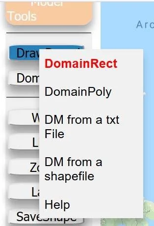
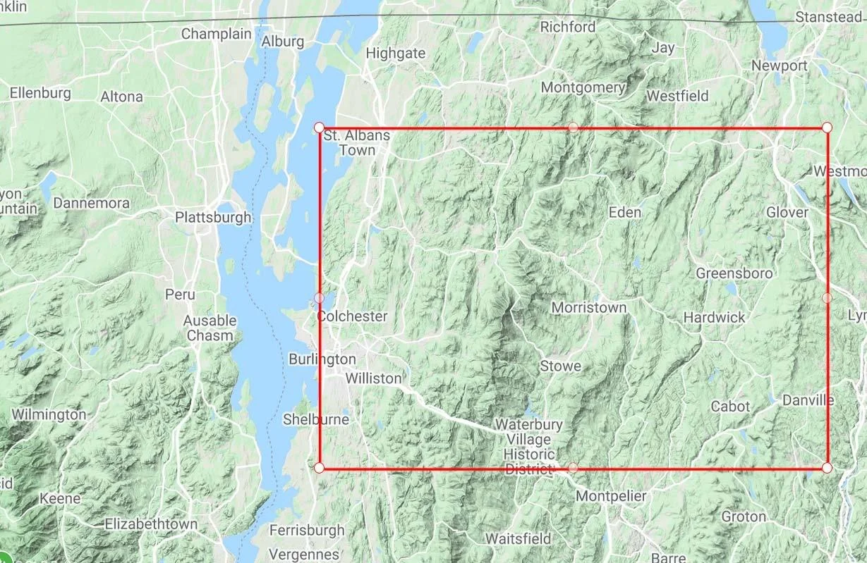
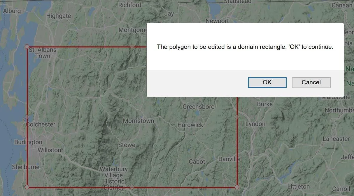
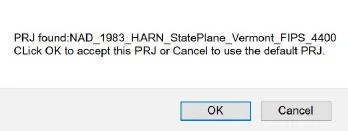
The moment you confirm your domain and accept the projection, a complete base model exists. The platform has already selected reasonable default values for every parameter: aquifer top from the Data Center DEM, aquifer bottom from minimum-DEM-minus-constant, hydraulic conductivity at a typical sand/gravel value, recharge at a typical humid-temperate value, porosity at 0.3, storage coefficients at reasonable defaults, and surface drainage active. You don't need to configure any of this to run a simulation. See Ch. 5 for what each parameter means and when to change defaults.
3.4 Click Simulate
The one-click moment. Everything you've done so far was setup; this is where you see the result.
Find the Simulate button
Look in the Simulation Tools panel — the second panel group in the toolbar. You'll see a button labeled Simulate.
Click it
The platform may ask you to log in again briefly (for server-side simulation credentials). Enter your password if prompted.
Wait a few seconds
For a 10 km × 10 km domain at default grid resolution, simulation typically takes 5 to 30 seconds. You'll see a progress indicator. If it takes longer than a minute, your domain is larger than expected or your internet connection is slow — both are fine, just wait.
For a standard rectangular domain with default settings, simulation rarely fails. If it does: (1) check that you drew the domain correctly — it should not cross a major coastline or include an obvious ocean area; (2) try a smaller domain; (3) verify your internet connection. If it keeps failing, open the Realtime-Help Reference from within the platform — the error message will have specific guidance.
3.5 Read What You See
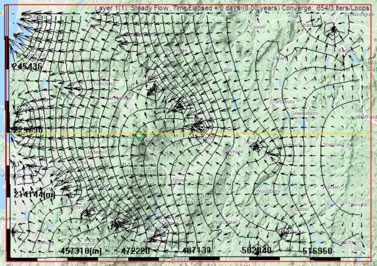
Simulation finished. Your map now shows the groundwater flow field for your site. Here's how to interpret what's on screen.
3.5.1 What the contours mean
The continuous lines on the map are hydraulic head contours — lines of equal groundwater elevation. They work the same way as topographic contours, except they show the water table, not the ground surface.
Key things to notice:
- Contours converge along rivers and lakes. Groundwater flows from high head to low head, perpendicular to the contour lines. Rivers and lakes act as drains — they are the local minima of the water-table surface.
- Contours diverge from highlands. Recharge areas — hills, ridges, interfluves — are where the water table is highest.
- Contour spacing reflects gradient. Tightly packed contours mean steep gradients (fast flow); widely spaced contours mean gentle gradients (slow flow).
3.5.2 What the vectors mean
The arrows are velocity vectors — each arrow shows the direction and magnitude of groundwater flow at a grid cell. Longer arrows mean faster flow.
Vectors always point from high head to low head, perpendicular to contour lines. Together, contours and vectors tell you the same story from two angles: contours are the "topography" of the water table; vectors are the flow on top of that topography.
3.5.3 A sanity check
Look at the contour and vector patterns. Do they make physical sense for your site?
- If your area has a river running through it, do you see head contours converging along the river? You should.
- If you know of major wetlands or springs, are they near local low points in the simulated water table? They should be.
- If your area includes a ridge or upland, is it a local high in the simulated water table? It should be.
If the answer to most of these is "yes," your base model is already telling you something true about your site — impressive given that you entered no site-specific parameters. If the answer is "no" for some questions, that's valuable too: those are the places refinement will matter most.
3.5.4 Explore the Analysis Tools
The flow field on the map is only one view. Click Analysis in the Analysis Tools panel to open a richer display:
- A 3D water-table surface — your aquifer visualized as a colored relief map
- A water balance — how much water enters and leaves your aquifer, broken down by source and sink
- A cross-section tool — draw a line on the plan view, see a vertical slice
- A legend — head values corresponding to the colors and contour lines
Take a minute to explore these. Each is self-explanatory once you see it.
3.6 Add Particles (Two Minutes More)
Head contours are static. Particles turn your model into a movie — you see water moving along its flow paths. This is where IGW-NET's "visual sandbox" philosophy becomes most vivid.
Open Particle Tools
In the Conceptual Model Tools panel, look for the particle-tracking buttons. Click ParticleRect (particle rectangle) to draw a grid of particle release points.
Draw a particle rectangle
Click-drag on the map to define a rectangular area. When you release, particles will be placed in a grid inside the rectangle. A good first choice: a rectangle covering a few cells near the upland edge of your domain, so particles have room to flow toward discharge features.
Choose forward or backward tracking
A dialog will ask whether you want forward tracking (particles move downstream with the flow) or backward tracking (particles trace upstream to their source). Choose forward for this first experience.
Click Simulate again
Particles are now part of your model. Re-simulate to see them animate along the flow field.
Head contours tell you where the water is; particles tell you where it goes. Watching a particle navigate from an upland recharge area, bend around a groundwater mound, and discharge into a river gives you an intuitive sense of flow paths that no static figure can match. Forward tracking answers "where does water from here end up?" Backward tracking answers "where did the water arriving here come from?" Both are central to wellhead protection, contamination source tracing, and understanding groundwater-ecosystem connections.
3.7 Save and What to Try Next
You have a working groundwater model. The last step is to save it so you can come back, and to know what to explore next.
3.7.1 Save your work
Click Save Model
In the File Tools panel, click Save Model. Give your model a name (e.g., "First Model — Lansing") and click OK. Your model is now stored on your MAGNET4WATER account and accessible from any browser where you log in.
Optional: download a local copy
For backup or sharing, click Download Model to save a model file to your local drive. You can later open this file in IGW-NET or email it to a colleague.
3.7.2 What you just did
In about 10–15 minutes, you:
- Created a complete, runnable groundwater flow simulation of a real site.
- Used high-resolution DEM data, typical aquifer parameters, and a robust default solver — all without knowing how any of this works internally.
- Got a first look at the groundwater flow field for your site.
- Explored particle tracking to see how water actually moves through the aquifer.
- Saved your work for future refinement.
This is the base model. Everything in this manual from here on is about refining it — making it more accurate, more site-specific, more useful for whatever question brought you to the platform in the first place.
3.7.3 Suggested next steps
| If you want to… | Read… |
|---|---|
| Understand what every aquifer-attribute default means | Ch. 5 — Aquifer Attributes (the conceptual heart of the manual) |
| Refine your model to a Data Center bedrock raster and K raster | Ch. 5 §5.2 — The customization ladder |
| Add rivers, lakes, and wells to your model | Ch. 6 — Features (Zones, Lines, Wells) |
| Compare with observations and calibrate | Ch. 17 — Calibration |
| Refine a specific local area without rebuilding | Ch. 13 — Nested Modeling (Submodels) |
| Model contaminant transport | Ch. 12 — Contaminant Transport |
| See what a real, published, calibrated model looks like | Case Study: Mancelona TCE Plume |
The moment from "never used the platform" to "I've built a working model" is the biggest learning hurdle for any groundwater tool. You've cleared it. Everything from here is refinement — adding detail, adding realism, adding specificity to your question. The platform will reward every hour you spend exploring it. Chapter 5 is where the real depth starts; the tutorials are where you'll pick up specific techniques; the case studies are where you'll see how it all comes together at real sites.
To go deeper
- Chapter 4 — Defining the Model Domain — your next chapter. More on domain choices: polygons, imported files, shapefiles, sizing decisions.
- Chapter 5 — Aquifer Attributes — the conceptual depth behind every default you just accepted.
- Quick Tutorial 1: 2D Steady Flow — the hands-on video-style version of this chapter.
- Quick Tutorial 3: Particle Tracking — more on forward and backward particle tracking.
- Concept: Fallback vs Spatial Values — the subtle but important thing you need to know about Data Center values.