Observe in Figure 5 the four green buttons on the left side of the modeling environment. Each of these yields a list box upon clicking. Figure 6 shows the contents of each List box. In setting up our model, we will normally begin with the top button in the left-most drop-down list. The DrawDomain button will be used to do just that, draw the domain or area of interest of our model (see Figure 7).
Since we first need to draw the domain, we click on this button to obtain the following four options. The first of these, DomainRect, will allow us to draw a rectangular domain very efficiently. This is the easiest choice and the one we will use. The DomainPoly option is an important alternative. It allows us to draw any polygonal area as the domain for our model. The next two, DM from a txt File and DM from a shapefile allow us to bring in information about our domain in a computer file when it is known, rather than actually drawing the domain with the mouse.
Since the map shown Figure 5 is at a very small scale we need to enlarge the scale to identify the area of interest for our model: the region around Burlington, Vermont. Let’s see how we move around this world map and change its scale. As long as the hand is visible over the map, double clicking and moving the hand moves the map (in some browsers, a single click-drag may suffice to move the map). If you use the mouse wheel to scroll, the map changes scale. We will first move the map to the general area we want to use for our model and then magnify the model to focus on the primary area of interest. We get the map shown in Figure 8.
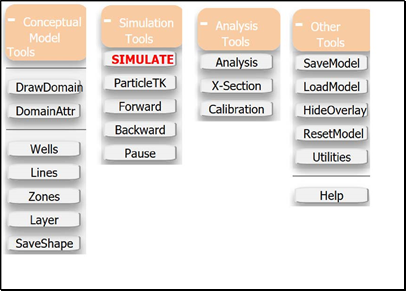
Figure 6: Tools for primary modeling activities.
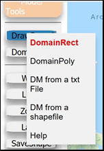
Figure 7: The rectangular drawing tool.
Next, we click on Conceptual Model Tools, then on the DrawDomain and finally on DomainRect as shown in Figure 7. When you move the mouse over the map area, you will see your mouse turn into a large plus sign. Place the mouse (plus sign) on a corner of the domain you want to create, say, for example the upper left-hand corner (northwest corner). Use a single left-mouse click to indicate the position of this first vertex of the rectangle. Then move the cursor to the location of the vertex that is diagonal from your initial vertex ("the opposite corner"). Use another LM click to place the vertices on the map - you will now see the domain rectangle; it will not appear after the first single click because the shape/size has yet to be defined at that point. Note that you should allow for a little bit of a pause in between left mouse clicks. If you click too quickly, it will be interpreted as a double-click which has a different meaning than single left mouse clicks. A double click will "zoom in" on the map display.
Now there are four corner points on the rectangle that will allow you to adjust its size and shape. The "little arrow" in the corner of the rectangle allows you to undo the last maneuver (one-step back only).
The next time you click anywhere inside the model domain you will get the window shown in Figure 10. Click OK to continue. You will be rewarded with another prompt (Figure 11) related to displaying display distances between vertices in the map display the next time you adjust the domain shape/size by dragging one of the vertices. Again, click OK. If you do this an undo button will appear next to it to reset the location to the previous position. Only the last position is kept in ‘MAGNET’s memory’. The message will disappear.
A second way to finalize the domain size and shape is to click the Conceptual Model Tools button and then click the SaveShape button. A third way is click on Other Tools and then on Utilities and finally on Geometry Locked. Both the 2nd and 3rd approach avoid the message prompts described in the previous paragraph.
At any time, you can change the shape/size of any geometry feature, including the model domain (or a zone feature or a line feature which we will discuss shortly), by click-dragging a node/vertex. But sometimes the geometry becomes "locked" (the nodes disappear). You can "unlock" the geometry by going to: Other Tools (button along the left-side of the Modeling environment) > Utilities > Geometry unlocked. If you want to hide the nodes, you can select the "Geometry Locked" option under utilities.
Note that, if you have an existing model domain and you click the DomainRect button, you will lose the existing domain. So it is better to use the Geometry unlocked button if you want to adjust the existing domain (rather than completely start over).
If you want to change your rectangle entirely go back to the DomainRect button and click it. The rectangle you just created will disappear and you start the process over. There is no universally applicable `undo’ button in this program. The idea for omitting the `undo’ button is justified because you can always click again the button you just clicked to get you to where you are and this will take you back to the beginning of the step that button initiated.
The possibility exists that you may want to move your map while the plus sign is replacing the cursor. To retrieve the hand you can click the 'SaveShape' button under "Conceptual Model Tools" to turn the cursor back to the "hand". If there was an "open" geometry feature (zone, line, or model domain), it will be "locked" by this action.
Note that, if you haven't started drawing anything (i.e., you haven't placed a vertex anywhere) the cursor will change back to a hand and there will not be any shapes (lines/zones) added to the map display.
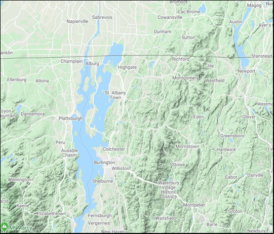
Figure 8: Area of interest for modeling.
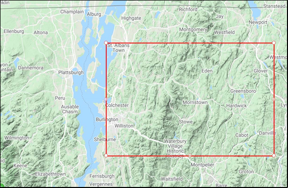
Figure 9: Rectangular area selected for model.
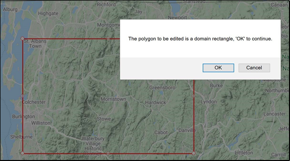
Figure 10: Response to selection of area of model.
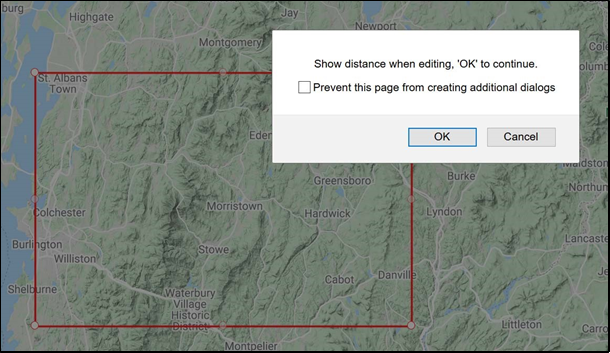
Figure 11: Second response window for definition of model boundaries.
Our model as shown in Figure 11 is actually a box that we are viewing from the top. By default the sides and bottom of our model (or box) as shown in Figure 11 are considered “no flow” boundaries (the top surface is a different story – more on that below). In other words, it is assumed there is no flux of groundwater across the sides or bottom boundaries of our model. However, unless a side boundary is aligned with a groundwater divide (which is hard to identify, and which changes in response to changes to recharge or pumping, for example), there may actually be some horizontal flow across these model boundaries. Therefore, the basic flow model we are developing may not be very accurate near the boundaries. But we can make the model large enough so that the area of interest is far from the boundary so the impacts of the no-flow conditions can be eliminated/minimized. Later we will learn how to use the basic model to provide boundary conditions (flow information) for a smaller, nested submodel with more details (see section 5).
As for the bottom of our model, the no flux boundary is normally identified with a geological layer that is of very low permeability. If there is no such layer, then a modification will need to be made to accommodate this flux and this is considered later.