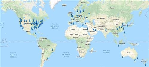
The Global Model Network is an open access repository of existing published MAGNET models, results, analyses, and visualizations. These models can be directly loaded and simulated in the MAGNET modeling environment for further customization and refinement. The Global Model Network functions essentially as a cyber-enabled observatory, allows teams composed of members from around the world to work on, analyze, and visualize the same model, live, in real time.
MAGNET users can choose to publish models (conceptual model, input parameters and time-series data), results, or part of their results. Other users can contact the model creator by commenting in model-specific chats, linking the groundwater community in new and exciting ways.
MAGNET users can choose to publish models (conceptual model, input parameters and time-series data), results, or part of their results. Other users can contact the model creator by commenting in model-specific chats, linking the groundwater community in new and exciting ways.
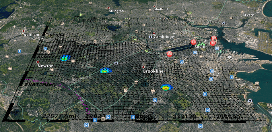


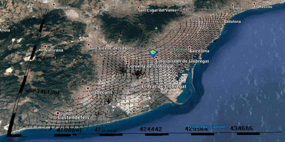
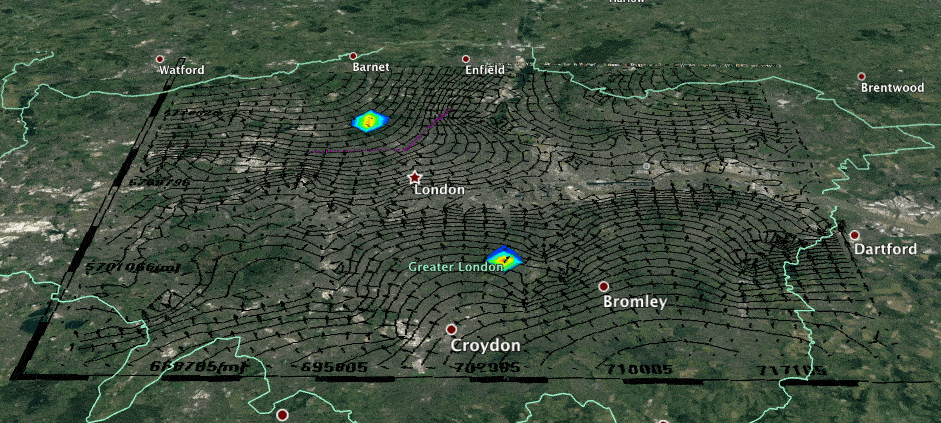
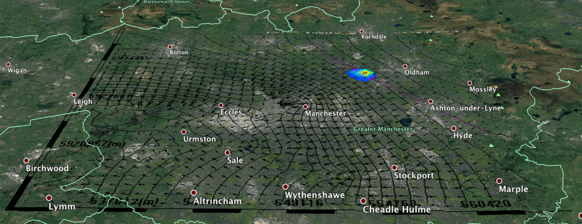
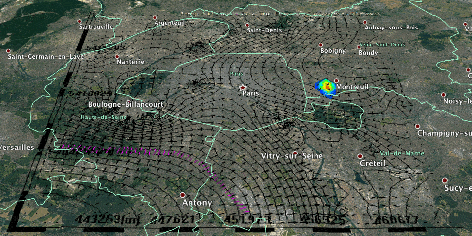
This model simulates natural groundwater conditions in the near-surface aquifer (i.e., the unconfined, water table aquifer) critical for water resource development and sustaining of groundwater-dependent ecosystems. Groundwater discharge into streams, lakes, wetlands, and springs - the major control of the long-term prevailing groundwater flow patterns - is captured through critical use of high-resolution Digital Elevation Models (DEMs). Specifically, the model predicts where the water table intersects the land surface as part of the solution process. In this way, the model generates qualitatively accurate head distributions (groundwater levels) needed to understand the near-surface environment and guide more detailed analysis and monitoring.
This model is not meant to be complete, but rather serve as a framework for customization - it is a preliminary, default model that can be modified, extended, and further customized based on study objectives and other available (local) data, as well as user experience and expertise.
Model Structure and Assumptions
Graphics/Animations
Model Improvement
Specific improvements that can be made include:
System-wide fine-tuning:
Adding Human Impacts:
Representing additional details:
Users are referred to the Magnet User Manual and Quick Tutorials available at www.magnet4water.com for additional details on implementing these improvements. Many of the tutorials can be completed almost instantly (with just a handful of buttons and keystrokes).
This model is not meant to be complete, but rather serve as a framework for customization - it is a preliminary, default model that can be modified, extended, and further customized based on study objectives and other available (local) data, as well as user experience and expertise.
Model Structure and Assumptions
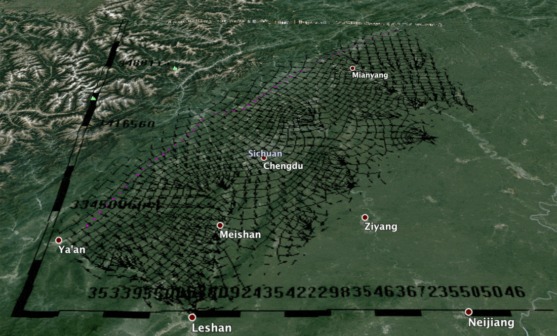
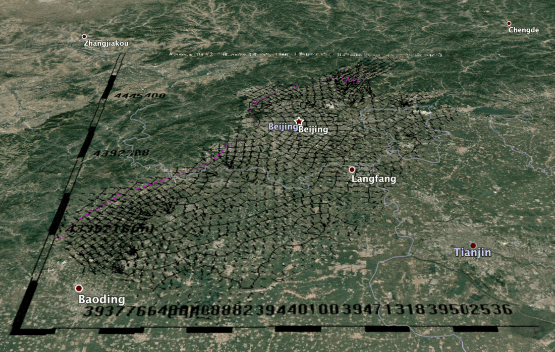
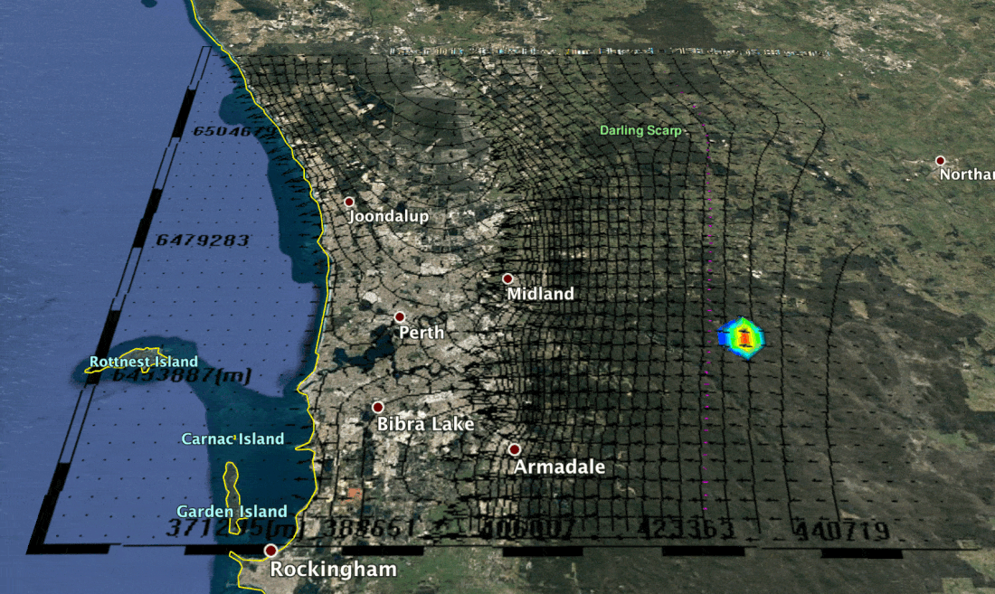
- The top of the aquifer is the spatially-variable land surface, represented by DEM (90 m resolution available globally from ASTER Global DEM, 30 or 10 m also available for United States from USGS NED).
- In instances where the groundwater head exceeds the land surface elevation, groundwater is allowed to leave the aquifer as a sink of water (i.e., groundwater is lost as surface seepage). This approach automatically captures the exchange of groundwater to surface water bodies as part of the robust solution process. By design, this approach does not allow infiltration of water from surface water bodies into the groundwater system, as prescribing boundary conditions of this nature requires careful application by the user, without which significant errors in the regional water balance can occur (even though the flow patterns may be correct).
- The bottom boundary is the top of the bedrock (where data is available), or computed as the minimum DEM elevation minus a user-prescribed length, Z (100 ft. in this instance). Users can easily apply different approaches as part of the model refinement process (see below).
- The bottom boundary is treated as a no-flow (zero groundwater flux across the boundary). This assumes the underlying consolidated sediments (bedrock) are practically impervious when compared to the overlying surficial aquifer, or little groundwater is exchanged between the geologic units. User can remove this assumption by explicitly modeling the bedrock layers below (see below).
- Lateral boundary conditions are also considered no-flow. The idea is to model a large enough area so that major regional recharge and discharge features are captured and the area of interest is sufficiently far from the boundaries as to not be impacted. Alternatively, a larger model can be solved first, and then this model can derive its lateral boundary conditions from the larger one (see below).
- Infiltration of precipitation on to the water table (groundwater recharge) is represented with a spatially variable raster based on prior studies or single, effective value for across the model domain, that can be modified by users based on local landscape, soil and climate conditions.
- The ease with which groundwater flows through the subsurface (hydraulic conductivity) is also represented with a spatially variable raster estimated based on water well lithologies (e.g., in Michigan) or is assumed as a single, effective value for across the model domain that can be modified by users.
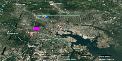
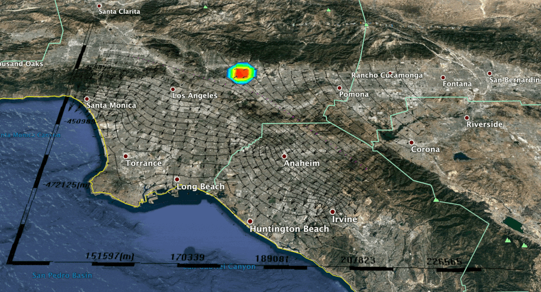
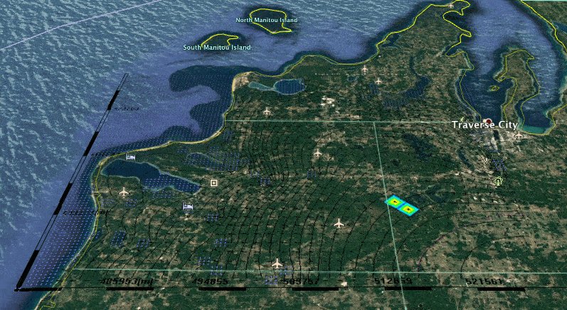
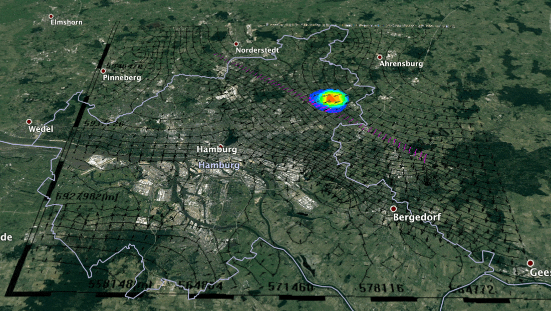
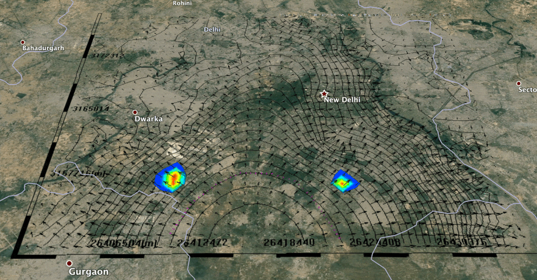
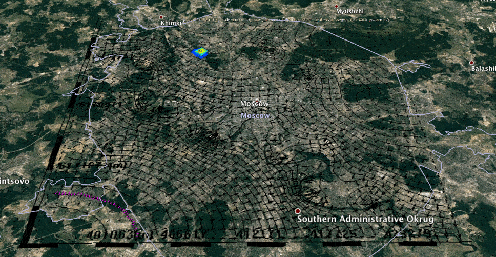
- Colored plumes are purely hypothetical and used solely for the purpose of illustrating how contaminants might move in the subsurface. They are assumed as surface sources, described by their source concentration and rate of infiltration into the aquifer.
Graphics/Animations
- the main area: water table elevation contours and concentration plumes originating from hypothetical sources
- pink particle lines: flow lines
- 3D surface plot: water table visualized as a 3D surface
- Concentration breakthrough curve or concentration as a function of time at the monitoring well
- Concentration profiles along the cross-section in different computational layers
- Water budget or summary of fluxes from different sources and sinks, in the model area
Model Improvement
Specific improvements that can be made include:
System-wide fine-tuning:
- Adjusting hydraulic conductivity based on knowledge of local geology, sedimentology, etc.
- Adjusting system-wide recharge based on knowledge of regional precipitation, primary land cover, etc.
- Improving the aquifer top (land surface) representation with user-provided DEMs (note that some areas may have erroneous/missing DEM patches, although this is a relatively rare occurrence).
- Changing the aquifer bottom elevation (bedrock top), or providing a spatially-variable input file
- Representing individual surface water bodies explicitly with prescribed head or flux boundary conditions used to describe exchange between groundwater and surface water
- Refining grid size (NX) to improve model resolution (x,y)
Adding Human Impacts:
- Adding pumping and/or injection wells
- Adding drain features and/or areas of artificial or restricted recharge
- Creating and customizing groundwater pollution sources
Representing additional details:
- Adding zones requiring a different hydraulic conductivity than the system-wide input.
- Subdividing the aquifer into multiple computational layers to provide greater vertical resolution of processes
- Adding 3D hydraulic conductivity heterogeneity for representing discrete geologic features as localized zones with upper and lower elevation limits (after subdividing into multiple computational layers)
- Adding additional aquifer layers for representing deeper geological units important to near-surface groundwater conditions (note that this is currently only available for MAGNET Premium - see magnet4water.com/Services).
- Adjusting the leakance (ease of flow) of if individual surface seeps and surface water bodies
- Developing a nested submodel that derives its boundary conditions from the current model in order to resolve finer spatial details
- Solving a larger model that can be used to provide boundary conditions for this model
Users are referred to the Magnet User Manual and Quick Tutorials available at www.magnet4water.com for additional details on implementing these improvements. Many of the tutorials can be completed almost instantly (with just a handful of buttons and keystrokes).